Dask kernel example
from dask.distributed import Client

client = Client("tcp://127.0.0.1:38150")
client
go to the dask array tab (shown below) and click on '<>'
from IPython.display import Image
Image(filename='./images/dask.png',width=400)
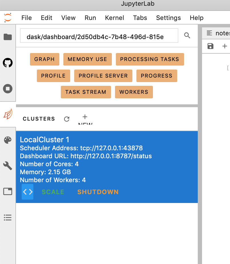
something similar to the cell below should have being incerted
from negi_stuff.modules.imps import (
    pd, np, xr, za, mpl, plt, sns, pjoin, os,
    glob, dt, sys, ucp, log, crt, cmip6
)
from pathlib import Path
df = cmip6.search_cmip6_hist(wildcard='mmrso4*',model='CESM*')
_ds = df.sort_values(['FORCING','REALIZATION'],ascending=[False,True])
_ds = df.sort_values(
    by       = [cmip6.FF,cmip6.RR,cmip6.FF],
    ascending= [False   ,True    ,True]
              )
_dg = _ds.groupby(cmip6.MODEL).first()
SIZE = 'SIZE'
df[SIZE] = df[cmip6.FILES].apply(lambda f: os.path.getsize(f))
_r = df.sort_values(SIZE, ascending=False).iloc[20]
_r['FILE_PATH']
large_file = '/home/28f6ea40-2d3059-2d4f6b-2d8429-2deb8e956423db/shared-cmip6-for-ns1000k/historical/CESM2/r11i1p1f1/mmrso4_AERmon_CESM2_historical_r11i1p1f1_gn_185001-189912.nc'
lets explore the dataset. however this is not opening the dataset as a [dask array] (https://examples.dask.org/xarray.html)
ds = xr.open_dataset(large_file)
#lets check the dimensions
ds.dims
#this will load the dataset as a dask array and therefore it will not kill the kernel
#some understanding of which operations you will perform on the dataset are needed
#in this case we are slicing the dataset along time in chunks of 1.
ds = xr.open_dataset(large_file,chunks={'time':1})
var = 'mmrso4'
# this will run fast but its just bc it hasn't been evaluated yet.
# so, daks will store the operations that you want on the dataset and only compute them
# when its necessary (e.g. when you want to plot the results). You can force the computation by
# calling .load() (see the next cell)
ds[var].mean()
# in order to get the actual value you need to load
# this will take some time since now we are actually computing the mean.
ds[var][{'time':slice(0,None)}].mean().load()
#convert cftime to datetime64
_c1 = ds['time'][0].item()
ds['time'] = pd.to_datetime(ds['time'].dt.strftime(_c1.format))
- first we average along the time dimension.
- then we load the results
- finally we copy the attrs for aesthaetics
da1 = ds[var].groupby('time').mean(xr.ALL_DIMS).load()
da1 = da1.assign_attrs(ds[var].attrs)
- we do a rolling mean.
- we use the results from the previous loading
da_rolling_mean = da1.rolling({'time':12*10},min_periods=1,center=True).mean()
da_rolling_mean = da_rolling_mean.assign_attrs(ds[var].attrs)
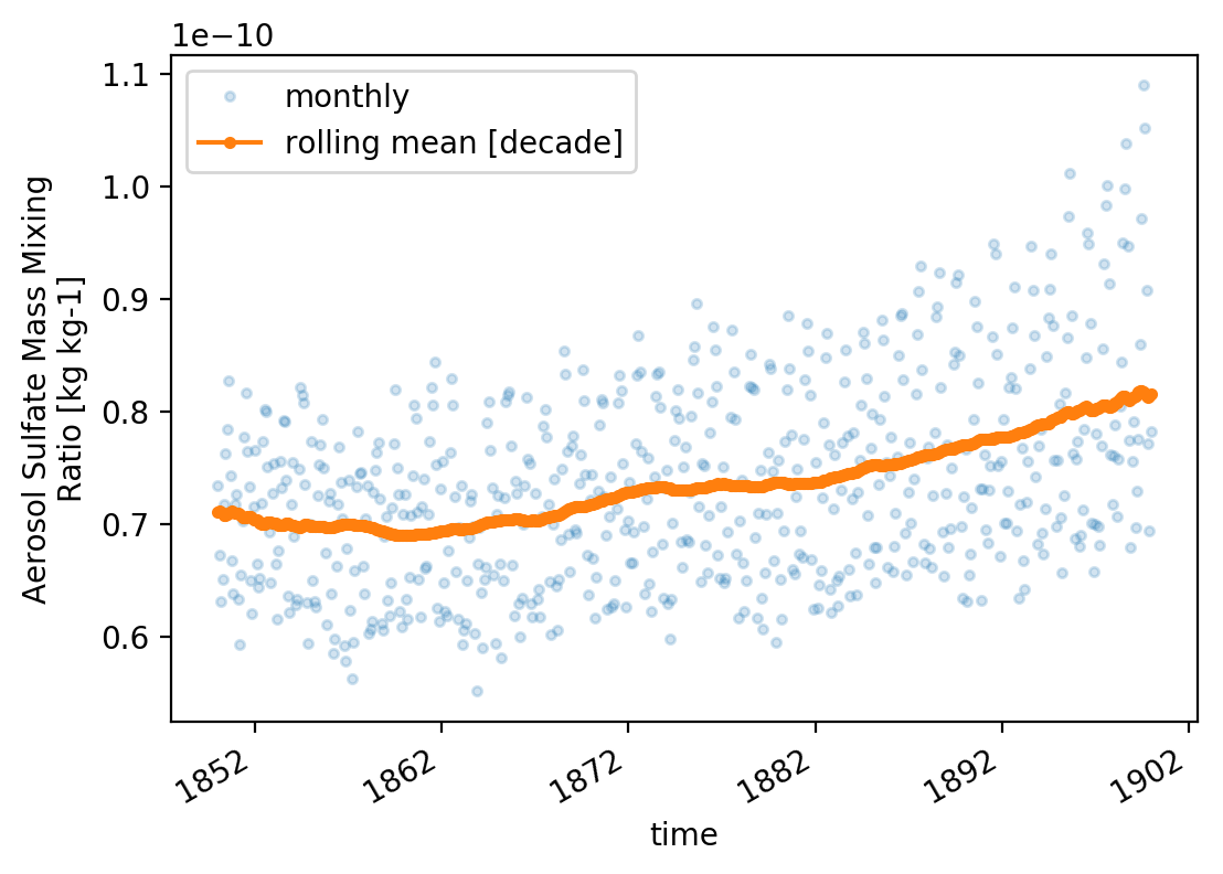
- define a function for plotting
def _plot():
    ax = plt.axes()
    l1 = 'monthly'
    l2 = f'rolling mean [decade]'
    da1.            plot(marker='.',linestyle='None', alpha=.2, label =l1, ax=ax )
    da_rolling_mean.plot(marker='.',linestyle='-'   , alpha=1 , label =l2, ax=ax )

    ax.legend();
_plot()
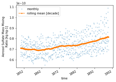
# increace res
mpl.rcParams['figure.dpi'] = 200
_plot()