import numpy as np
import matplotlib.pyplot as plt
from netCDF4 import Dataset
import xarray as xr
import pandas as pd
import cartopy.crs as ccrs
import datetime

!wget https://zenodo.org/record/3475894/files/Abisko-prep.tar.gz

!tar zxvf Abisko-prep.tar.gz

#observations
Stoffel = pd.read_csv('Abisko-prep/T_recon_NTREND_NH1_EURO.csv', index_col='Year')

#check data
Stoffel

#check shape
Stoffel.shape

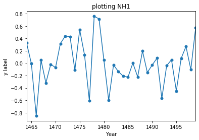
Stoffel['NH1'].plot()

starty=1464; endy=1500
ax = Stoffel['NH1'].loc[range(starty,endy)].plot(title = 'plotting NH1', marker='.', markersize=10)
ax.set_ylabel("y label")

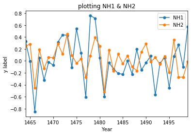
starty=1464; endy=1500
ax = Stoffel[['NH1','NH2']].loc[range(starty,endy)].plot(title = 'plotting NH1 & NH2', marker='.', markersize=10)
ax.set_ylabel("y label")

#open control run
cntrl = xr.open_dataset('Abisko-prep/piControl_BOT_1850-2849_temp2_fldmean.nc', decode_times  = True, use_cftime = True)

# set reference time so it makes it easier to use with xarray
!cdo setreftime,1850-01-31,00:00:00 Abisko-prep/piControl_BOT_1850-2849_temp2_fldmean.nc Abisko-prep/po.nc

cntrl = xr.open_dataset('Abisko-prep/po.nc', decode_times  = True, use_cftime = True)

cntrl.time.values

cntrl.var167
# Same as specifying cntrl['var167']

#Go from Kelvin to Celsius
cntrl['var167'] = cntrl['var167']-273.15

cntrl

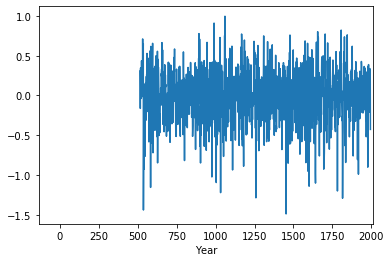
cntrl['var167'].plot()

std_cntrl = cntrl['var167'].groupby('time.month').std().mean()
#For a 2 sigma std
sig2 = std_cntrl*2
sig2

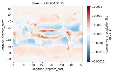
ds_ens = xr.open_dataset('Abisko-prep/ensmean_PE_seas.nc')
ds_ens

ds_ens['aprc'].isel(time=1).plot()

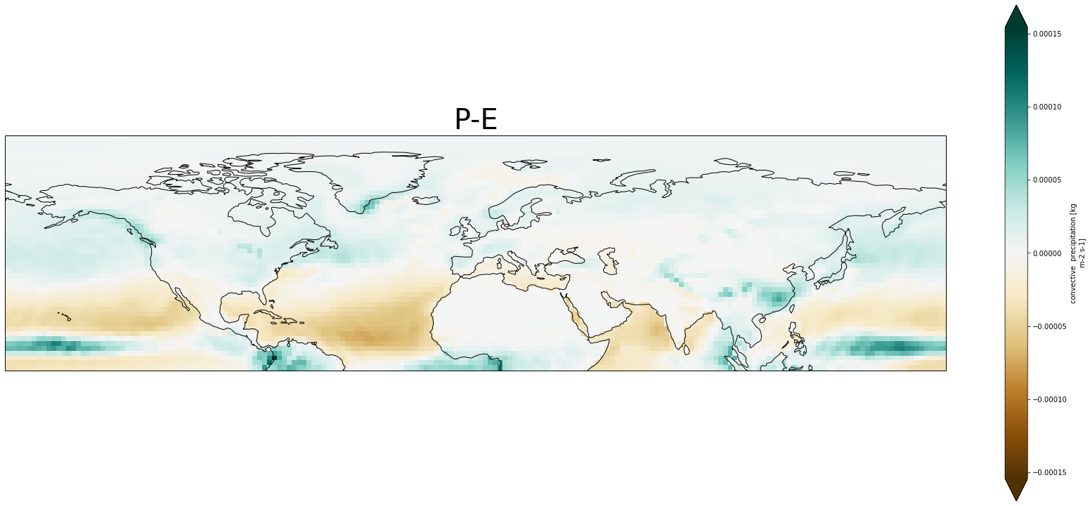
#plot maps
#For maps you take the ensemble mean
fig = plt.figure(1,figsize = [30,13])

#range
vc=np.arange(-2,3,.5)

# We're using cartopy and are plotting in PlateCarree projection 
# (see documentation on cartopy)
ax1 = plt.subplot(1, 1, 1, projection=ccrs.PlateCarree())
ax1.coastlines()

ds_ens['aprc'].isel(time=1).plot.pcolormesh(ax = ax1, extend='both', cmap=plt.get_cmap('BrBG'))
#Title
plt.title('P-E', fontsize=40)
#If you want you can zoom in to a specific area
ax1.set_xlim([-180,180])
ax1.set_ylim([0,90])

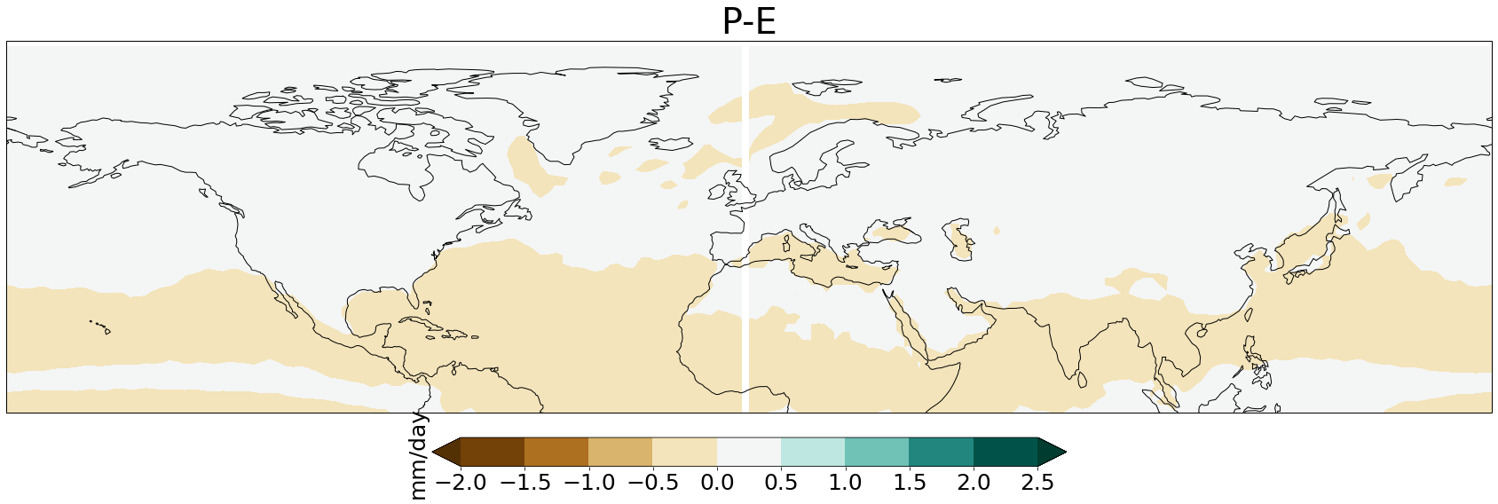
#plot maps
#For maps you take the ensemble mean


fig = plt.figure(1,figsize = [30,13])

#range
vc=np.arange(-2,3,.5)

# We're using cartopy and are plotting in PlateCarree projection 
# (see documentation on cartopy)
ax1 = plt.subplot(1, 1, 1, projection=ccrs.PlateCarree())
ax1.coastlines()
map=ax1.contourf(ds_ens['lon'][:], ds_ens["lat"][:], ds_ens['aprc'][0,:,:],vc, 
                 extend='both', cmap=plt.get_cmap('BrBG'))

#Title
plt.title('P-E', fontsize=40)
#If you want you can zoom in to a specific area
ax1.set_xlim([-180,180])
ax1.set_ylim([0,90])

#plotting a colorbar
cbar = plt.colorbar(map, extend='both', orientation='horizontal', fraction=0.046, pad=0.04)
cbar.ax.tick_params(labelsize=25)
cbar.ax.set_ylabel('mm/day', fontsize=25)

#To get rid of the white line in the middle --> shift white to the edges of the map
data = ds_ens['aprc']

shifted = np.zeros_like(data.data)
shifted.shape

half = 96
shifted[:,:, 0:96] = data.data[:,:, 96:]
shifted[:,:, 96:] = data.data[:, :, :96]

data.data = shifted
data.lon.data -= 180
data.lon

fig = plt.figure(1,figsize = [30,13])
vc=np.arange(-2,3,.5)

ax1 = plt.subplot(1, 1, 1, projection=ccrs.PlateCarree())
ax1.coastlines()
map=ax1.contourf(ds_ens['lon'][:], ds_ens["lat"][:], ds_ens['aprc'][0,:,:],vc, extend='both', cmap=plt.get_cmap('BrBG'))

plt.title('P-E', fontsize=40)

cbar = plt.colorbar(map, extend='both', orientation='horizontal', fraction=0.046, pad=0.04)
cbar.ax.tick_params(labelsize=25)
cbar.ax.set_ylabel('mm/day', fontsize=25)

ds_ens_a = xr.open_dataset('Abisko-prep/ensmean_1536_1550_geopoth_seas_a.nc')

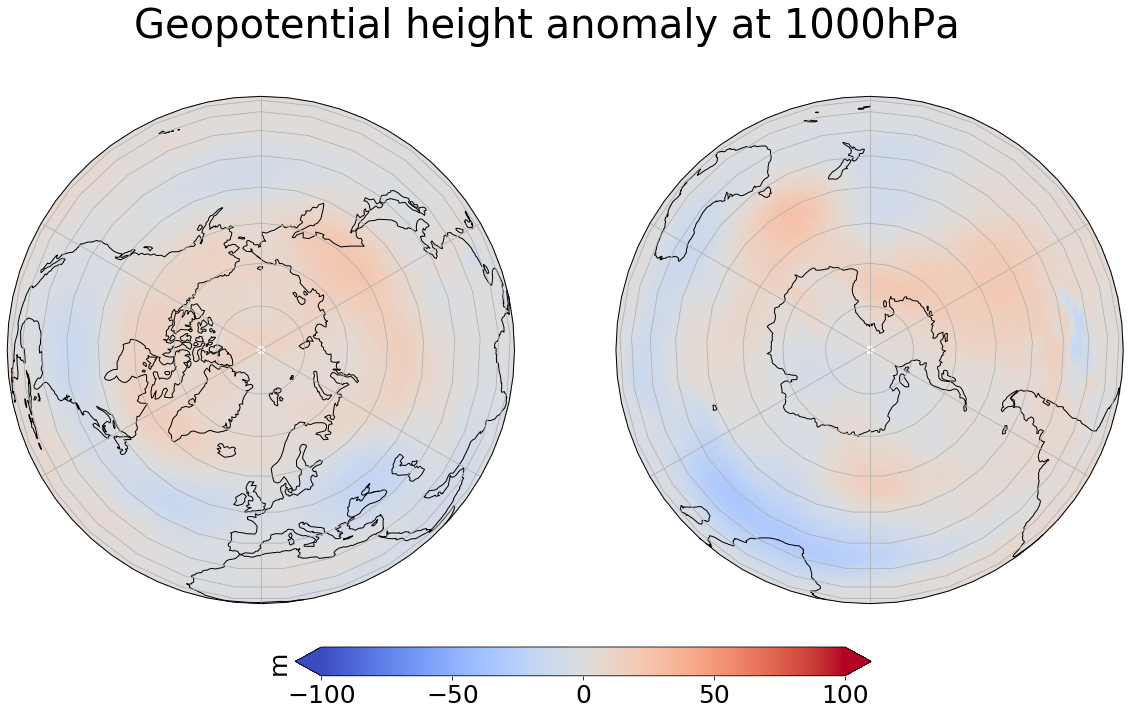
#Other projections are for example Orthographic projection

fig = plt.figure(figsize=[20, 10])

img = ds_ens_a['var156'][64,0,:,:]
crs = ccrs.PlateCarree()
extent = ([-180, 180, -90, -60], ccrs.PlateCarree())

# ax1 for Northern Hemisphere
ax1 = plt.subplot(1, 2, 1, projection=ccrs.Orthographic(0, 90))

# ax2 for Southern Hemisphere
ax2 = plt.subplot(1, 2, 2, projection=ccrs.Orthographic(180, -90))

for ax in [ax1, ax2]:
    ax.coastlines()
    ax.gridlines()
    map = ax.imshow(img, vmin=-100, vmax=100, transform=crs, cmap=plt.get_cmap('coolwarm'))

#Titel for both plots
fig.suptitle('Geopotential height anomaly at 1000hPa', fontsize=40)

cb_ax = fig.add_axes([0.325, 0.05, 0.4, 0.04])

cbar = plt.colorbar(map, cax=cb_ax, extend='both', orientation='horizontal', fraction=0.046, pad=0.04)
cbar.ax.tick_params(labelsize=25)
cbar.ax.set_ylabel('m', fontsize=25)

plt.show()

#plot timeseries --> open climate model data ensemble runs + ensemble mean
#for a timeseries we need to have global average data --> CDO fldmean (area weighted)
ds_tas_01_a_trees_yr = xr.open_dataset('Abisko-prep/ue536a01_temp2_pre_seas_trees_fldmean_a_yrmean.nc')
ds_tas_02_a_trees_yr = xr.open_dataset('Abisko-prep/ue536a02_temp2_pre_seas_trees_fldmean_a_yrmean.nc')
ds_tas_03_a_trees_yr = xr.open_dataset('Abisko-prep/ue536a03_temp2_pre_seas_trees_fldmean_a_yrmean.nc')
ds_tas_04_a_trees_yr = xr.open_dataset('Abisko-prep/ue536a04_temp2_pre_seas_trees_fldmean_a_yrmean.nc')
ds_tas_05_a_trees_yr = xr.open_dataset('Abisko-prep/ue536a05_temp2_pre_seas_trees_fldmean_a_yrmean.nc')
ds_tas_06_a_trees_yr = xr.open_dataset('Abisko-prep/ue536a06_temp2_pre_seas_trees_fldmean_a_yrmean.nc')
ds_tas_ens_a_trees_yr = xr.open_dataset('Abisko-prep/ensmean_temp2_pre_seas_trees_fldmean_a_yrmean.nc')

#plot timeseries --> obs and ds in same plot
#Create time array
time_yr = time = np.arange('0526-01-31', '0552-01-28', dtype='datetime64[Y]')

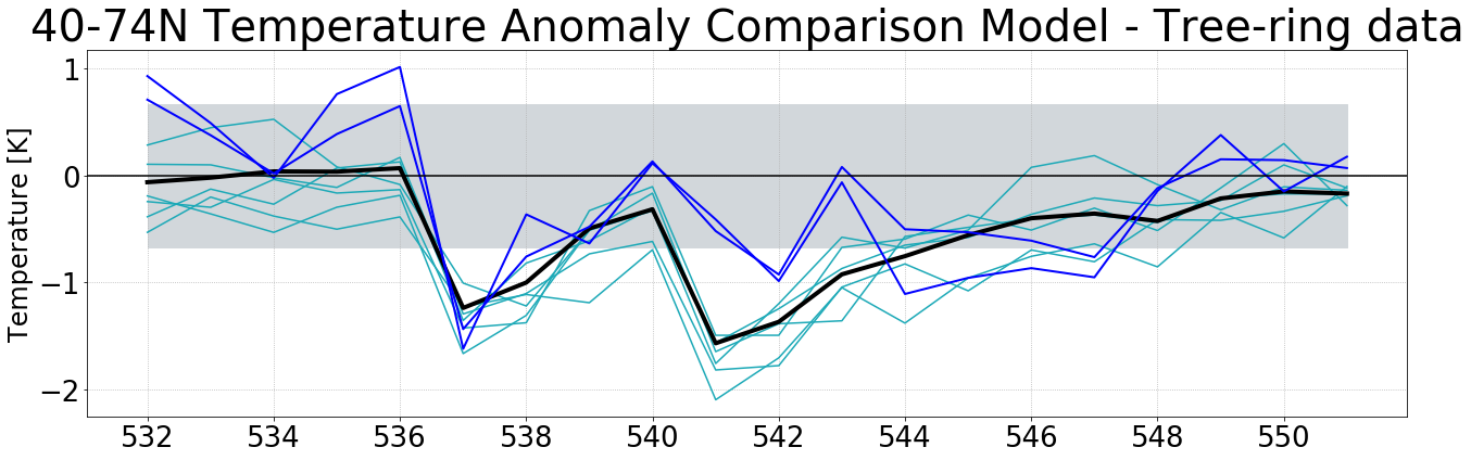
#plot timeseries --> obs and ds in same plot

fig = plt.figure(12, figsize= (20,6))

#Ensemble runs and ensemble mean 
plt.plot(time_yr[6:], ds_tas_01_a_trees_yr['temp2'][6:,0,0], label = 'run01', color = '#1ca9b7')
plt.plot(time_yr[6:], ds_tas_02_a_trees_yr['temp2'][6:,0,0], label = 'run02', color = '#1ca9b7')
plt.plot(time_yr[6:], ds_tas_03_a_trees_yr['temp2'][6:,0,0], label = 'run03', color = '#1ca9b7')
plt.plot(time_yr[6:], ds_tas_04_a_trees_yr['temp2'][6:,0,0], label = 'run04', color = '#1ca9b7')
plt.plot(time_yr[6:], ds_tas_05_a_trees_yr['temp2'][6:,0,0], label = 'run05', color = '#1ca9b7')
plt.plot(time_yr[6:], ds_tas_06_a_trees_yr['temp2'][6:,0,0], label = 'run06', color = '#1ca9b7')

plt.plot(time_yr[6:], ds_tas_ens_a_trees_yr['temp2'][6:,0,0], label = 'ensmean', color = 'black', linewidth = 4 )

#Observational data
#Make sure the data has the same shape and the time axis is the same. In this case we had to flip the data because it
#went back in time in the obs dataset
plt.plot(time_yr[6:], np.flip(Stoffel['NH1'][1464:1484]), label = 'NH1', color = '#0000FF', linewidth = 2)
plt.plot(time_yr[6:], np.flip(Stoffel['NH2'][1464:1484]), label = 'NH2', color = '#0000FF', linewidth = 2)

#Have a line at 0
plt.axhline(0, color='black')

#Std
plt.fill_between(time_yr[6:],-0.6723, 0.6723, color = '#d2d7db')#std control run 

#grid
plt.grid(linestyle=':')

#Titel
plt.title('40-74N Temperature Anomaly Comparison Model - Tree-ring data', fontsize=40)

#label y-axis
plt.ylabel('Temperature [K]', fontsize=24)

#size of the ticks
plt.tick_params(labelsize=26)

plt.tight_layout()

#save figure
#plt.savefig('figures/seasonal_temp_a_timeseries_trees_2sig_treeringdata.png', bbox_inches = 'tight')

plt.show()

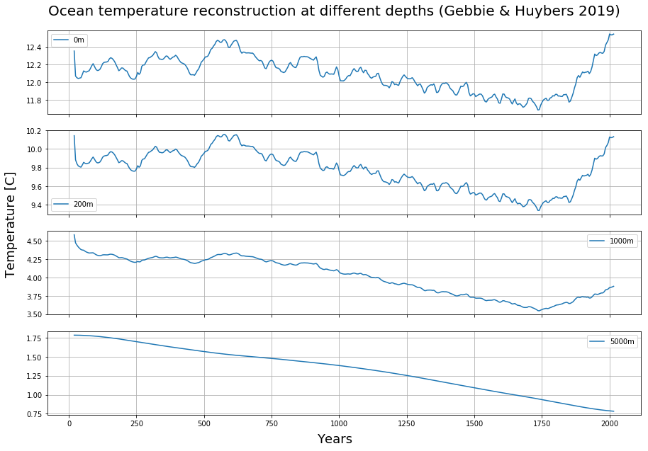
ds = xr.open_dataset('Abisko-prep/Theta_OPT-0015.nc')

ds_timeseries = np.mean(ds['theta'], axis=(0,1))

#Plot subplots
fig, axs = plt.subplots(4, figsize=(15,10), sharex=True)


axs[0].plot(ds['year'], ds_timeseries[0,:], label='0m')
axs[0].grid()
axs[0].legend()


axs[1].plot(ds['year'], ds_timeseries[8,:], label='200m')
axs[1].grid()
axs[1].legend()

axs[2].plot(ds['year'], ds_timeseries[17,:], label='1000m')
axs[2].grid()
axs[2].legend()

axs[3].plot(ds['year'], ds_timeseries[-2,:], label='5000m')
axs[3].grid()
axs[3].legend()

fig.suptitle('Ocean temperature reconstruction at different depths (Gebbie & Huybers 2019)',x=0.5, y=0.93, ha='center', 
             va='top', fontsize=20)
fig.text(0.07, 0.5, 'Temperature [C]', va='center', rotation='vertical', fontsize=18)
fig.text(0.5, 0.07, 'Years', ha='center', fontsize=18)