Plotting CMIP6 data
!wget http://esgf-data.ucar.edu/thredds/fileServer/esg_dataroot/CMIP6/CMIP/NCAR/CESM2/historical/r1i1p1f1/Amon/tas/gn/v20190308/tas_Amon_CESM2_historical_r1i1p1f1_gn_185001-201412.nc
filename = 'tas_Amon_CESM2_historical_r1i1p1f1_gn_185001-201412.nc'
import xarray as xr
import cartopy.crs as ccrs
import matplotlib.pyplot as plt
import numpy as np
import cftime
dset = xr.open_dataset(filename, decode_times=True, use_cftime=True)
print(dset)
print(dset['tas'])
dset.time.values
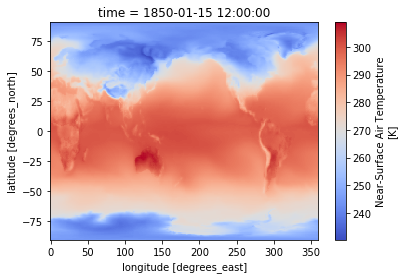
dset['tas'].sel(time=cftime.DatetimeNoLeap(1850, 1, 15, 12, 0, 0, 0, 2, 15)).plot(cmap = 'coolwarm')
- select the nearest time. Here from 1st April 1950
dset['tas'].sel(time=cftime.DatetimeNoLeap(1850, 4, 1), method='nearest').plot(cmap='coolwarm')
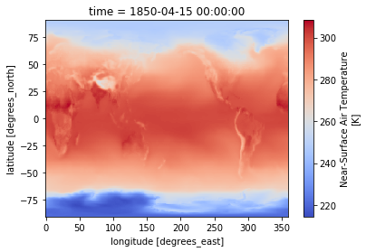
fig = plt.figure(1, figsize=[30,13])

# Set the projection to use for plotting
ax = plt.subplot(1, 1, 1, projection=ccrs.PlateCarree())
ax.coastlines()

# Pass ax as an argument when plotting. Here we assume data is in the same coordinate reference system than the projection chosen for plotting
# isel allows to select by indices instead of the time values
dset['tas'].isel(time=0).plot.pcolormesh(ax=ax, cmap='coolwarm')
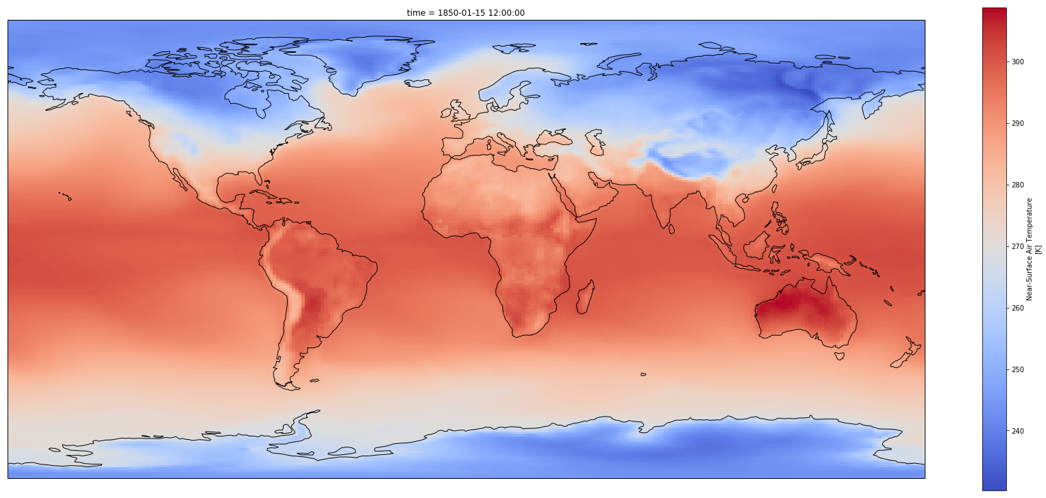
fig = plt.figure(1, figsize=[10,10])

# We're using cartopy and are plotting in Orthographic projection
# (see documentation on cartopy)
ax = plt.subplot(1, 1, 1, projection=ccrs.Orthographic(0, 90))
ax.coastlines()

# We need to project our data to the new Orthographic projection and for this we use `transform`.
# we set the original data projection in transform (here PlateCarree)
dset['tas'].isel(time=0).plot(ax=ax, transform=ccrs.PlateCarree(), cmap='coolwarm')

# One way to customize your title
plt.title(dset.time.values[0].strftime("%B %Y"), fontsize=18)
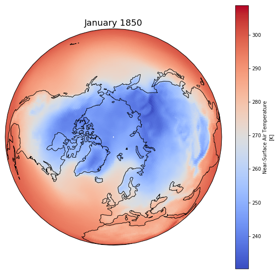
fig = plt.figure(1, figsize=[10,10])
ax = plt.subplot(1, 1, 1, projection=ccrs.Orthographic(0, 90))
ax.coastlines()
# Fix extent
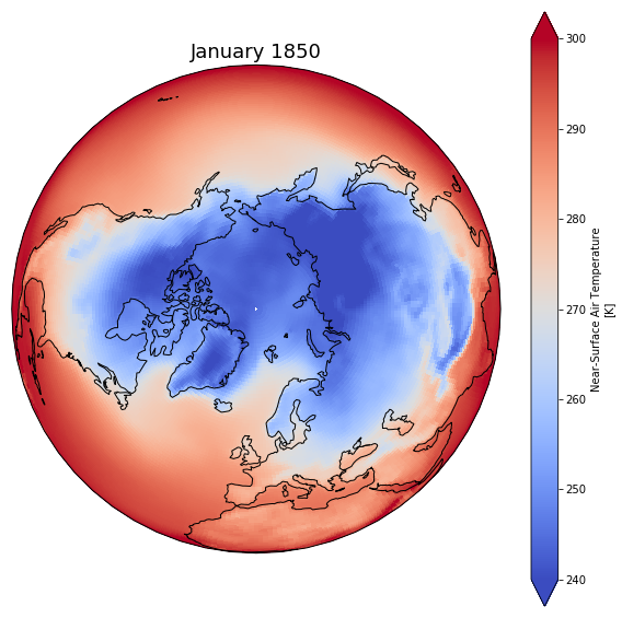
minval = 240
maxval = 300
# pass extent with vmin and vmax parameters
dset['tas'].isel(time=0).plot(ax=ax, vmin=minval, vmax=maxval, transform=ccrs.PlateCarree(), cmap='coolwarm')
# One way to customize your title
plt.title(dset.time.values[0].strftime("%B %Y"), fontsize=18)
proj_plot = ccrs.Orthographic(0, 90)

p = dset['tas'].sel(time = dset.time.dt.year.isin([1850, 2014])).plot(x='lon', y='lat',
                                                                 transform=ccrs.PlateCarree(),
                                                                 aspect=dset.dims["lon"] / dset.dims["lat"],  # for a sensible figsize
                                                                 subplot_kws={"projection": proj_plot},
                                                                 col='time', col_wrap=6, robust=True, cmap='PiYG')
# We have to set the map's options on all four axes
for ax,i in zip(p.axes.flat,  dset.time.sel(time = dset.time.dt.year.isin([1850, 2014])).values):
    ax.coastlines()
    ax.set_title(i.strftime("%B %Y"), fontsize=18)
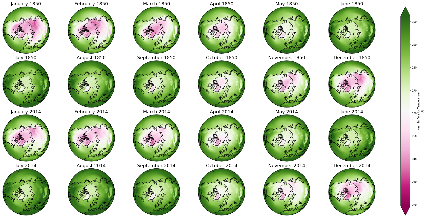
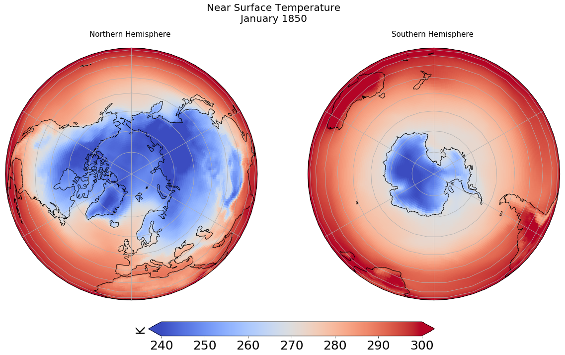
fig = plt.figure(1, figsize=[20,10])

# Fix extent
minval = 240
maxval = 300

# Plot 1 for Northern Hemisphere subplot argument (nrows, ncols, nplot)
# here 1 row, 2 columns and 1st plot
ax1 = plt.subplot(1, 2, 1, projection=ccrs.Orthographic(0, 90))

# Plot 2 for Southern Hemisphere
# 2nd plot
ax2 = plt.subplot(1, 2, 2, projection=ccrs.Orthographic(180, -90))

tsel = 0
for ax,t in zip([ax1, ax2], ["Northern", "Southern"]):
    map = dset['tas'].isel(time=tsel).plot(ax=ax, vmin=minval, vmax=maxval,
                                           transform=ccrs.PlateCarree(),
                                           cmap='coolwarm',
                                           add_colorbar=False)
    ax.set_title(t + " Hemisphere \n" , fontsize=15)
    ax.coastlines()
    ax.gridlines()

# Title for both plots
fig.suptitle('Near Surface Temperature\n' + dset.time.values[tsel].strftime("%B %Y"), fontsize=20)


cb_ax = fig.add_axes([0.325, 0.05, 0.4, 0.04])

cbar = plt.colorbar(map, cax=cb_ax, extend='both', orientation='horizontal', fraction=0.046, pad=0.04)
cbar.ax.tick_params(labelsize=25)
cbar.ax.set_ylabel('K', fontsize=25)