
Intercomparison between CMIP6 models, MERRA2 satellite-retrieved reanalysis data and AERONET of aerosol optical depth
Franziska Hellmuth NEGI course 2019 - eScience for linking Arctic measurements and modeling Group assistants: Paul Glantz, Ksenia Tabakova, Jonas Gliss
Abstract
We compare aerosol optical depth (AOD) from 12 Coupled Model Intercomparison Project 6 (CMIP6) models with Modern-Era Retrospective analysis for Research and Applications 2 (MERRA2) and ground-based observational data from the AErosol RObotic NETwork (AERONET) in the Arctic and zonally. We find that MERRA2 satellite reanalysis is too high compared to the Sunphotometer measurements. Seasonal variation of AOD over the last 34 years was mostly not reproduced by the 12 CMIP6 models. CanESM5 and GFDL-CM4 simulated AOD values within the MERRA2 variability during Arctic spring. MERRA2 reanalysis shows a decrease of AOD in the Northern Hemisphere since 1980. GFDL-ESM4 and GFDL-CM4 simulated the zonally averaged AOD within the MERRA2 reanalysis. NorESM-LM2 has too much sea salt in the Southern Hemisphere (50$^\circ$S) and too little AOD above 40$^\circ$N. Further work has to be done to clarify the contribution and representation of sea salt in NorESM-LM2.
Introduction
It has long been known that the Arctic region is particularly sensitive to global warming (Collins et al., 2013). Atmospheric Aerosols are particles suspended in the air. Some Aerosols have been produced by natural processes others by human activities. Aerosols in the Atmosphere reduce the amount of incoming solar radiation by scattering or absorbing light of solar radiation. The amount of atmospheric Aerosols varies with location, time and due to events such as dust storms, forest fires and volcanic eruptions (Lohmann et al., 2016). In a warming climate, will the sea ice decrease and larger areas of open water will follow an increase in organic aerosol uptake. Aerosols (natural or anthropogenic) can affect the Earth climate through interaction with solar radiation and clouds. Aerosol optical depth (AOD) is a measure of the amount of sunlight that has been scattered or absorbed.
The largest ground-based AOD measurement project is the AErosol RObotic NETwork (AERONET). The Sunphotometers are distributed over the globe and can give information about the distribution of aerosols in the atmosphere. This measurements are sparse and represent the AOD distribution only for a small area. With the launch of satellites, it is possible to retrieve global estimates of aerosol optical depth. Cloud free daily data can be used to reanalyse the AOD in a finer grid-scale and use it to validate global climate model performance to predict the changing climate more accurately.
Glantz et al., 2014 analysed the AOD in the Svalbard area. They compared Moderate Resolution Imaging Spectroradiometer (MODIS) Aqua retrievals of AOD to Sunphotometer measurements from Svalbard. The study shows that the Svalbard region undergoes a seasonal cycle with higher AOD during spring and a low AOD during summer. The remote sensing data is then used to examine the AOD generation of global climate models, represented in the Coupled Model Intercomparison Project 5 (CMIP5). In the 1980 - 2014 period show the CMIP5 models an underestimation of AOD during spring and an overestimation during summer when compared to remote sensing data.
In the presented study nine years of Modern-Era Retrospective analysis for Research and Applications 2 (MERRA2), satellite reanalysis is compared to ground-based Sunphotometer AOD measurements in the Arctic. Afterwards, are climate model simulations from CMIP6 examined in comparison to MERRA2 satellite reanalysis over 34 years.
The following questions have been addressed:
- How representative are MERRA2 satellite reanalysis in comparison to the ground-based AOD observations in the Arctic?
- How accurately does the global climate models of CMIP6 simulate the AOD for the Arctic and zonally for the last three decades?
Section 2.1 and Section 2.2 contains the code to read the observational data from the Sunphotmeters and the MERRA2 satellite reanalysis in the Arctic region, respectively. Section 2.3 consists of the code for finding the AOD at 550nm in the CMIP6 models and their ensembles. Section 3 will then present the results to answer the questions above.
Ground-based, satellite reanalysis and CMIP model data
Global climate models are essential to study future climate changes of aerosols and clouds.
Aerosol optical depth (AOD) at 550nm from Sunphotometer measurements from Aerosol Robotic Network (AERONET) is used as the reference to satellite retrieved reanalysis MERRA2. Then, AOD satellite reanalysis is utilised with comparable aerosol properties from historical Phase 6 of the CMIP6 model runs. The CMIP6 includes 33 participating model groups (Eyring et al., 2016) and data is available through the CMIP6 search interface https://esgf-data.dkrz.de/search/cmip6-dkrz/. Of these 33 models, we focus on twelve models to evaluate the AOD. The model specifications can be found in Table 1.
| Resolution | Vertical levels | Top level | Version | Time Range | References | Identifier | ||
|---|---|---|---|---|---|---|---|---|
| (lat x lon) | (nominal) | |||||||
| CanESM5 | 2.8$^\circ$ x 2.8$^\circ$ | 500 km | 49 | 1 hPa | 2019-05-03 | 1980 - 2014 | Swart et al., 2019 | 10.22033/ESGF/CMIP6.3610 |
| CESM2 | 0.9$^\circ$ x 1.25$^\circ$ | 100 km | 32 | 2.25 hPa | 2019-01-16 | 1980 - 2014 | NCAR CESM2, 2018 | 10.22033/ESGF/CMIP6.7627 |
| CESM2-WACCM | 0.9$^\circ$ x 1.3$^\circ$ | 100 km | 70 | 4.5x10$^{-6}$ hPa | 2019-01-30 | 1980 - 2014 | NCAR CESM2, 2018 | 10.22033/ESGF/CMIP6.10071 |
| CNRM-CM6-1 | 1.4$^\circ$ x 1.4$^\circ$ | 250 km | 91 | 0.01 hPa | 2018-06-20 | 1980 - 2014 | Voldoire et al., 2019 | 10.22033/ESGF/CMIP6.4066 |
| E3SM-1-0 | 1.0$^\circ$ x 1.0$^\circ$ | 100 km | 72 | 0.1 hPa | 2019-07-24 | 1980 - 2014 | Golaz et al., 2019 | 10.22033/ESGF/CMIP6.4497 |
| GFDL-CM4 | 1.0$^\circ$ x 1.2$^\circ$ | 100 km | 33 | 1 hPa | 2019-02-23 | 1980 - 2014 | Held et al., 2019 | 10.22033/ESGF/CMIP6.8594 |
| GFDL-ESM4 | 1.0$^\circ$ x 1.2$^\circ$ | 100 km | 49 | 0.01 hPa | 2019-08-06 | 1980 - 2014 | 10.22033/ESGF/CMIP6.8597 | |
| IPSL-CM6A-LR | 1.27$^\circ$ x 2.5$^\circ$ | 250 km | 79 | 40.000 m | 2018-07-11 | 1980 - 2014 | 10.22033/ESGF/CMIP6.5195 | |
| MIROC-ES2L | 2.8$^\circ$ x 2.8$^\circ$ | 500 km | 40 | 3 hPa | 2019-06-25 | 1980 - 2014 | Hajima et al., 2019 | 10.22033/ESGF/CMIP6.5602 |
| MPI-ESM1-2-HR | 1.0$^\circ$ x 0.9$^\circ$ | 100 km | 95 | 0.01 hPa | 2019-08-25 | 1980 - 2014 | 10.22033/ESGF/CMIP6.6594 | |
| NorESM2-LM | 1.9$^\circ$ x 2.5$^\circ$ | 250 km | 32 | 3 hPa | 2019-08-15 | 1980 - 2014 | Kirkevåg et al., 2018 | NCC.NorESM2-LM.historical |
| Sunphotometer AERONET | 2006 - 2014 | Giles et al., 2019 | ||||||
| MERRA2 | 0.5$^\circ$ x 0.65$^\circ$ | 72 | 0.01 hPa | 5.12.4 | 1980 - 2014 | Gelaro et al., 2017 |
### Create dask cluster to work parallel in large datasets

from dask.distributed import Client
client = Client(n_workers=2,
                threads_per_worker=2,
                memory_limit='2GB',
                processes=False)
client
chunks={'time' : 10,}
client
# supress warnings
import warnings
warnings.filterwarnings('ignore') # don't output warnings

# Import packages
from franzihe_imports import (xr, plt, np, ccrs, sns, pd, pya, fct, )
from glob import (glob)
pya.change_verbosity('critical', log=pya.const.print_log)
pya.__version__


# reload imports
%load_ext autoreload
%autoreload 2


# Plotting cosmetics
fct.plot_style()

# save figures to ./Figures/ folder
savefig = 0     # 1 = yes, 0 = no
### Define data location for AERONET Sunphotometer, MERRA2 and CMIP6

pyaero_path = 'shared-ns1000k/inputs/pyaerocom-testdata'
merra_path  = 'data_MERRA2/'
cmip_path   = 'shared-cmip6-for-ns1000k/historical/'
AERONET Sunphotometer
I want to read in the AOD measured at 550nm by the Sunphotometer for the Arctic region. The definition for the Arctic region is latitudes larger than 66$^\circ$N.
I will transform it into xarry since its functionality will make it easier for me to handle the data. Plotting is similar as in pandas. The function read_aerocom_return_xarray_median_std will help me to read in the station data with Pyaerocom. The output will give the AOD at 550nm, the longitude and latitude, median and standard deviation for the Arctic stations. Most of the stations had a course data coverage, therefore, did I decide to use the years 2006 to 2014.
# Pick out the stations for the Arctic
# Lat in decimal form
lower_lat = 66.; lower_lon = -180.
upper_lat = 90.; upper_lon = 180.
# Pick out the years for analysis
starty = '2006'
endy   = '2014'

# AeroCom AOD values from Arctic stations
aeronet_arctic = fct.read_aerocom_return_xarray_median_std(pyaero_path, lower_lat, upper_lat, starty, endy)

# only use AERONET stations which have data for starty and endy
valid_aeronet_arctic = {}
for station_name in aeronet_arctic.keys():
    if len(aeronet_arctic[station_name]['median_'+starty+endy]) <= 0 or \
       len(aeronet_arctic[station_name]['std_'+starty+endy]) <= 0:
        continue
    else:
        valid_aeronet_arctic[station_name] = aeronet_arctic[station_name]
        print(station_name,
              valid_aeronet_arctic[station_name]['latitude'],
              valid_aeronet_arctic[station_name]['longitude'])
MERRA2
In Section 3.1, the MERRA2 satellite reanalysis is evaluated against the ground-based AOD measurements to know how representative MERRA2 is for the Arctic stations. For this we used NASAs GIOVANNI interface to retrieve the monthly AOD averages for the stations. All MERRA2 data is the Aerosol Optical Depth at 550nm from MODIS. The processed analysis value is marked with M2IMNXGAS.
We chose the grid box closest to the latitude and longitude of the AERONET stations in the Arctic.
The function read_merra2_return_xarray_median_std will read in the .csv files according to the station latitude and longitude from AERONET and returns a xarray. A monthly median and standard deviation is created for the AOD values to analyse the seasonal variability in Fig. 2 for 2006 - 2014.
# MERRA2 AOD values from Arctic stations
_mfile = merra_path + 'g4.areaAvgTimeSeries.M2IMNXGAS_5_12_4_AODANA.2006'
merra_arctic = fct.read_merra2_return_xarray_median_std(aeronet_arctic, _mfile, starty, endy)
MERRA2 satellite reanalysis has monthly averages of AOD from 1980. This values will be used to evaluate the CMIP6 historical simulations for the Arctic region (latitudes larger than 66$^\circ$N). The historical simulations help to evaluate the performance of the models against observations and provides insight into future projections.
The function read_merra2 will return a pandas DataFrame.
# Arctic 180W,66N - 180E,90N (1980-2014)
_mfile = merra_path+ 'g4.areaAvgTimeSeries.M2IMNXGAS_5_12_4_AODANA.19800101-20141231.180W_66N_180E_90N.csv'
merra_hist = fct.read_merra2(_mfile, 'mean_M2IMNXGAS_5_12_4_AODANA', 'M_Arctic' )
merra_hist.head()
I also started analysing a region west of Svalbard against the ground-based station Hornsund . Therefore will this region be added to the pandas.DataFrame.
# Nordic Sea, west of Svalbard 15W,75N - 10E,82N
_mfile = merra_path+ 'g4.areaAvgTimeSeries.M2IMNXGAS_5_12_4_AODANA.19800101-20141231.15W_75N_10E_82N.csv'

merra_hist.insert(loc=1,
                  column='M_Svalbard',
                  value=fct.read_merra2(_mfile, 'mean_M2IMNXGAS_5_12_4_AODANA', 'M_Svalbard' )['M_Svalbard'].values)
merra_hist.head()
To make the plotting easier, later on, will I transfer the pandas.DataFrame to xarray for the Arctic and Svalbard region.
# add to merra arctic xarray stations the Arctic area(180W-180E,66-90N) and
# the Svalbard area (15W-10E,75-82N)

merra_arctic['M_Arctic'] = {}
merra_arctic['M_Svalbard'] = {}
merra_arctic['M_Arctic']['od550aer'] = xr.DataArray(merra_hist['M_Arctic'], dims=['time',])
merra_arctic['M_Svalbard']['od550aer'] = xr.DataArray(merra_hist['M_Svalbard'], dims=['time',])
The Arctic AOD values are averaged to present the seasonal variability of MERRA2 data. Fig. 1 to Fig. 3 use monthly averages over several years to present this. calc_xarray_median_std will calculate the median for the stations and the Arctic region, 2006 - 2014 and 1980 - 2014, respectively.
# median and std for 2006-2014
merra_arctic['M_Arctic'] = fct.calc_xarray_median_std_monthly(merra_arctic['M_Arctic'],'od550aer', '2006', '2014')
# median and std for 1980-2014
merra_arctic['M_Arctic'] = fct.calc_xarray_median_std_monthly(merra_arctic['M_Arctic'],'od550aer', '1980', '2014')
Fig. 5 will evaluate twelve CMIP6 models against MERRA2, zonally for three decades (1980s, 1990s, 2000s). The NASA GIOVANNI interface already provides a zonal mean for AOD at 550nm.
read_merra2_zonal will read the .csv files and returns a dictonary containing the xarray for each decade.
# find zonal csv files
fn_list = glob(merra_path+'g4.zonalMean.M2IMNXGAS_5_12_4_AODANA.*')
fn_list.sort()
fn_list

# read zonal files and assign to dictonary with xarray
_dir = merra_path+'g4.zonalMean.M2IMNXGAS_5_12_4_AODANA.*'
#merra_zonal = fct.read_merra2_zonal(_dir)

_dir = merra_path+'g4.dimensionAveraged.M2IMNXGAS_5_12_4_AODANA.19800101-20141231.180W_90S_180E_90N.nc'
merra_zonal = xr.open_dataset(_dir)

# calculate the media and standard deviation of each decade and all years
merra_zonal = fct.calc_xarray_median_std_yearly(merra_zonal, 'M2IMNXGAS_5_12_4_AODANA', '1980', '1989')
merra_zonal = fct.calc_xarray_median_std_yearly(merra_zonal, 'M2IMNXGAS_5_12_4_AODANA', '1990', '1999')
merra_zonal = fct.calc_xarray_median_std_yearly(merra_zonal, 'M2IMNXGAS_5_12_4_AODANA', '2000', '2009')
merra_zonal = fct.calc_xarray_median_std_yearly(merra_zonal, 'M2IMNXGAS_5_12_4_AODANA', '1980', '2014')
Information about the correlation between MERRA2 and the AERONET stations will be helpful to validate how representative the MERRA2 reanalysis is compared to the Arctic stations.
calc_statistic uses a function from Pyaerocom, namely pyaerocom.mathutils.calc_statistics. It will return all necessary values to analyse the correlation.
stat_arctic_st, stat_arctic_merra = fct.calc_statistic(aeronet_arctic, merra_arctic, '2006', '2014')
_hmd = glob(cmip_path+'/*')
cmip6_model = []       # find all model names of historical runs
for i in range(len(_hmd)):
    cmip6_model.append(_hmd[i][len(cmip_path):])
print('CMIP6 models containing AOD at 550nm')
print(*cmip6_model, sep = ',')
After returning all CMIP6 models, I will now search in the subfolders containing the AOD at 550nm.
For each model, monthly data from 1980 - 2014 is chosen to overlap with MERRA2. There are several ensembles and realisations available. I use the r1i1p1f1, r1i1p2f1, r1i1p1f2 ensemble member, as it was available on the shared-cmip6-for-ns1000k folder.
Read all CMIP6 historical simulation including the AOD at 550nm (1980-2014) with read_all_cmip6_od550aer. The function will return a dictionary containing the model name and ensemble member. The longitude is shifted from originally 0-360$^\circ$ to 180$^\circ$W - 180$^\circ$E. Areacella values are added to the xarray to later calculate the weighted averages with the masked_average function (provided by assistants on NEGI-2019 webpage).
cmip = fct.read_all_cmip6_od550aer(cmip6_model,cmip_path,chunks,
                                   lower_lat, upper_lat,
                                   lower_lon, upper_lon, '1980', '2014')
In this step, the weighted averages for each CMIP6 model and ensemble member are performed for chosen years and chosen region. First, I will evaluate the CMIP6 models in the Arctic region (latitude larger than 66$^\circ$N) between 1980 and 2014. The function calc_weighted_av_median_std will add to the existing cmip dictionary the weighted average for AOD as well as the monthly median and standard deviation for the chosen period.
starty='1980'; endy='2014'

# calculate weighted mean, monthly mean and standard deviation for the Arctic
for model in cmip.keys():
    for rea in cmip[model].keys():
        cmip[model][rea] = fct.calc_weighted_av_median_std(cmip[model][rea],
                                                           starty, endy,
                                                           model,
                                                           cmip[model][rea]['lat'] <= (lower_lat-5),
                                                           ['lat', 'lon'],
                                                           lower_lat, upper_lat,
                                                           lower_lon, upper_lon,
                                       )
# only use cmip data which have data for starty and endy and average to a monthly mean
valid_cmip={}
for model in cmip.keys():
    valid_cmip[model] = {}
    for rea in cmip[model].keys():
        try:
            cmip[model][rea]['median_'+starty+endy]
            valid_cmip[model][rea] = cmip[model][rea]
        except KeyError:
            continue
Fig. 4 is analysing the AOD zonally against MERRA2. Weighted averages have to be created zonally for the CMIP historical simulations for each decade to make it comparable.
for model in cmip.keys():
    for rea in cmip[model].keys():
        # for 1980-1989
        cmip[model][rea]  = fct.calc_weighted_av_median_std(cmip[model][rea],
                                                            '1980','1989',
                                                            model,
                                                            dim=['lon'])
        # for 1990-1999
        cmip[model][rea]  = fct.calc_weighted_av_median_std(cmip[model][rea],
                                                            '1990','1999',
                                                            model,
                                                            dim=['lon'])
        # for 2000-2009
        cmip[model][rea]  = fct.calc_weighted_av_median_std(cmip[model][rea],
                                                            '2000','2009',
                                                            model,
                                                            dim=['lon'])
# get only the model keys for models which are used in the study
_mm = []
_rr = []
for model in valid_cmip.keys():
    if len(valid_cmip[model].keys()) > 0:
        if len(valid_cmip[model].keys()) >=1:
            for rea in valid_cmip[model].keys():
                _mm.append(model)
                _rr.append(rea)
Results and Discussion
As mentioned before, CMIP6 historical simulations will be evaluated against the satellite reanalysis product MERRA2. To have confidence in the analysis, the MERRA2 AODs are compared to the AERONET ground-based stations Section 3.1. With a warming climate, the areas of open water will increase in the Arctic. Related to this will the sea-salt and organic aerosol discharge increase (Glantz et al., 2014). The Arctic undergoes a seasonal cycle of AOD. During the Arctic summer new particle formation occurs due to higher insolation $\rightarrow$ higher levels of OH and more efficient precipitation cleansing. Section 3.2 will evaluate the CMIP6 seasonal cycle in the Arctic region between 1980 and 2014. The zonal assessment of CMIP6 models will then give an insight into how the models simulated the past three decades in a 'global' scale (Section 3.3).
# Figure 1
numfig = 1
starty = '2006'; endy = '2014'
fig = plt.figure(figsize=[30,10])
ax1 = fig.add_subplot(131,
                      projection= ccrs.AzimuthalEquidistant(central_longitude=0,
                                                            central_latitude=90,))

ax2 = fig.add_subplot(132)
ax3 = fig.add_subplot(133)
for station_name, i  in zip(valid_aeronet_arctic.keys(), range(len(valid_aeronet_arctic))):
        # Plot stations on map
        ax1.plot(valid_aeronet_arctic[station_name]['longitude'],
                 valid_aeronet_arctic[station_name]['latitude'],
                 'o',
                 color = sns.color_palette("hls",len(valid_aeronet_arctic))[i],
                 markersize=20,
                 transform=ccrs.PlateCarree(),
                 label=station_name)
        ax1.annotate(station_name[0:3], xy=(valid_aeronet_arctic[station_name]['longitude']+0.15, valid_aeronet_arctic[station_name]['latitude']+0.15),
                     xycoords=ccrs.PlateCarree()._as_mpl_transform(ax1),
                    ha='right', va='top', fontsize=20)
        # Sunphotometer vs MERRA2 at stations
        fct.plt_scatter(aeronet_arctic[station_name]['median_'+starty+endy],
                        merra_arctic[station_name]['median_'+starty+endy][int(aeronet_arctic[station_name]['median_'+starty+endy][0].month-1):int(aeronet_arctic[station_name]['median_'+starty+endy][-1].month)],
                        [0.015,0.8],[0.015,0.8],
                        'AOD$_{median}$ Aeronet Sunphotometer (550nm)', 'AOD$_{median}$ MERRA2 at stations (550nm)',
                        stat_arctic_st,
                        'b)', ax2, sns.color_palette("hls",len(valid_aeronet_arctic))[i])
        # MERRA2 Arctic median vs MERRA2 at stations
        fct.plt_scatter(merra_arctic['M_Arctic']['median_'+starty+endy],
                        merra_arctic[station_name]['median_'+starty+endy],
                        [0.015,0.8],[0.015,0.8],
                        'AOD$_{median}$ MERRA2 Arctic (550nm)', 'AOD$_{median}$ MERRA2 at stations (550nm)',
                        stat_arctic_merra,
                        'c)', ax3, sns.color_palette("hls",len(valid_aeronet_arctic))[i])

# Limit the map degrees latitude
ax1.set_extent([-180, 180, 90, 60], ccrs.PlateCarree())
ax1.coastlines()
ax1.gridlines()
ax1.set_title('a)', fontweight='bold')


# Legend
ax3.legend(bbox_to_anchor=(1.1, 1.05));

if savefig == 1:
    filename = './Figures/AOD_station_correlation.png'
    plt.savefig(filename,#transparent=True,
                bbox_inches='tight');
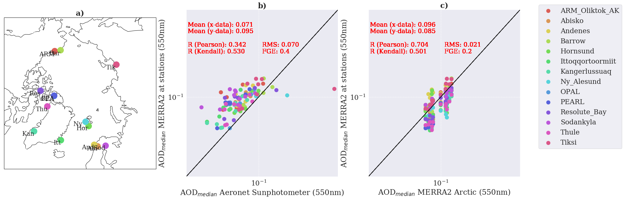
In Fig. 1a) we see valid measurement stations for AOD in the Arctic region between 2006 and 2014. The monthly medians of AOD at the stations are present in Fig. 1b). MERRA2 comparison on how well the AOD at the stations is in comparison to the Arctic area-averaged AOD shows in Fig. 1c). The linear Pearson correlation coefficient for all stations is +0.3 (Fig. 1b)), meaning the data points are varying from the best fit and having a medium correlation. We also see that MERRA2 overestimates the monthly mean AOD. With this in mind, we compare the two MERRA2 data sets, Fig. 1c). The correlation is large (R$_{Pearson}$ = 0.7), but not best. However, this result will give us later some confidence when we are analysing the CMIP6 historical simulations.
We want to see further how well the MERRA2 Arctic median compares to the AERONET ground-based measurements, in particular, the seasonal variation of AOD. Therefore monthly means for each station are plotted together with the MERRA2 data described in Section 2.2. The study focuses only on the summer months and on cloud-free days, where measurements at the AERONET station existed.
# Figure 2
starty = '2006'; endy = '2014'
fig, axsm = plt.subplots(2,7, sharex='all', sharey='all',
                         figsize = [30,10])
axs = axsm.flatten()
for station_name, i  in zip(valid_aeronet_arctic.keys(), range(len(valid_aeronet_arctic))):

        # plot aeronet monthly median at station
        fct.plt_seasonal_model_ensemble(valid_aeronet_arctic[station_name], axs[i],
                                        starty, endy,
                                        sns.color_palette("hls",len(valid_aeronet_arctic))[i])
        # plot MERRA2 monthly median at station
        fct.plt_seasonal_model_ensemble(merra_arctic[station_name], axs[i],
                                        starty, endy,
                                        'darkblue')
        # plot MERRA monthly median for Arctic
        fct.plt_seasonal_model_ensemble(merra_arctic['M_Arctic'], axs[i],
                                        starty, endy,
                                        'k')

        axs[i].set_title(station_name, color=sns.color_palette("hls",len(valid_aeronet_arctic))[i],fontweight='bold')
        axs[i].set_xlim([2,10])
        axs[i].set_ylim([0, 0.25])
        axs[i].set_xticks(np.arange(2,11))
#        axs[i].set_ylabel('AOD (550nm)')
        axs[i].set_ylabel('')
        axs[i].set_xlabel('')

axs[0].set_ylabel('AOD (550nm)')
axs[7].set_ylabel('AOD (550nm)')
for i in range(7,14):
    axs[i].set_xlabel('Month')


axs[len(valid_aeronet_arctic)-1].legend(['AERONET', 'MERRA2$_{Station}$', 'MERRA2$_{Arctic}$'],
                                        bbox_to_anchor=(1.1, 1.05), loc='lower left', borderaxespad=0., fancybox=True)
plt.subplots_adjust(wspace = 0.2, hspace=0.4)
fig.suptitle('%s - %s, median and $\sigma$' %(starty, endy),
            fontsize=28,fontweight='bold');

if savefig == 1:
    filename = './Figures/station_AERONET_MERRA2.png'
    plt.savefig(filename,#transparent=True,
                bbox_inches='tight');
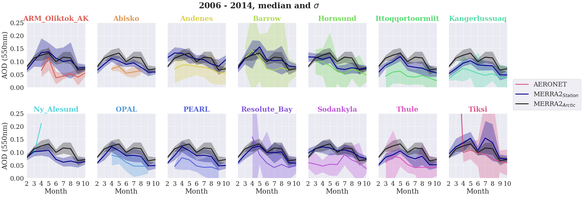
The coloured lines in Fig. 2 represent the monthly medians from the AERONET stations between 2006 and 2014. Most of the ground-based observations show an AOD peak during spring, except Andenes (Norway) and Sodankyla (Finnland). The spring peak is likely associated with Arctic haze events. Arctic haze events are an occasionally enhanced Arctic aerosol loading by continental aerosols from midlatitudes. Furthermore, marine aerosols can have contributed to higher observed AOD due to the enhanced production by surface wind speeds during spring (Glantz et al., 2014).
Abisko (Sweden), Barrow (Alaska), Hornsund (Svalbard), Ittoqqortoormiit (Greenland) and Sodankyla (Finnland) show a peak during Arctic summer. From 2006 to 2014 was the Arctic highly influenced by aerosols from volcanic eruptions, such as Kasatochi (Alaska), Sarychev (Russia) and Nabro (Africa) in August 2008, July 2009 and June 2011, respectively. Furthermore, large agricultural fires in Eastern Europe and Canada resulted in an increase of AOD in the Arctic Region (Glantz et al., 2014).
Besides at the PEARL station (Northern Canda), none of the MERRA2 station data represents the seasonal cycle well. In all cases is the satellite reanalysis too high in comparison to the ground-based measurements.
MERRA2 station AOD averages are lower compared to the Arctic average for 50% of the stations, namely Abisko (Sweden), Hornsund (Svalbard), Ittoqqortoormiit (Greenland), Kangerlussuaq (Greenland), Ny Ålesund (Svalbard), OPAL, PEARL (Northern Canada), Thule (Greenland).
For all stations, we have to keep in mind that I only focused on the months with daylight and cloud-free days for AERONET and MERRA2 measurements and reanalysis, respectively.
CMIP6 seasonal evaluation
The previous finding will be helpful for the assessment of the CMIP6 historical simulations between 1980 and 2014. We have to keep in mind, that the seasonal variation of AOD for the Arctic region is only partly representative for the AERONET stations where MERRA2 showed almost everywhere too high values. Furthermore, the MERRA2 AOD at 550nm is always too high when compared to the ground-based observations.
# Figure 3
handles = {}
starty = '1980'; endy   = '2014'
xtick_label = ['Jan', 'Feb', 'Mar', 'Apr', 'May', 'Jun', 'Jul', 'Aug', 'Sep', 'Oct', 'Nov', 'Dec']
fig, axsm = plt.subplots(1,2, sharex = 'row', sharey='all',
                       figsize=[30,10])
axs = axsm.flatten()

# plot the MERRA2 seasonal cycle
handles['M_Arctic'] = fct.plt_seasonal_model_ensemble(merra_arctic['M_Arctic'], axs[0],  starty, endy,'k', label='MERRA2' )
fct.plt_seasonal_model_ensemble(merra_arctic['M_Arctic'], axs[1],  starty, endy,'k' )
# plot CMIP6 seasonal cycle
for model, rea, i in zip(_mm[:int(len(_mm)/2)], _rr[:int(len(_rr)/2)], range(int(len(_mm)/2))):
    l1 = fct.plt_seasonal_model_ensemble(valid_cmip[model][rea], axs[0], starty, endy,
                                          sns.color_palette("Paired",12)[i], label=model+'_'+rea)

    handles[model+'_'+rea] = l1

axs[0].set_ylabel('AOD (550nm)')
axs[0].set_title('')
axs[0].set_ylim([0,0.175])


for model, rea, i in zip(_mm[int(len(_mm)/2):], _rr[int(len(_rr)/2):], range(int(len(_mm)/2), len(_mm))):
    handles[model+'_'+rea] = fct.plt_seasonal_model_ensemble(valid_cmip[model][rea], axs[1], starty, endy,
                                          sns.color_palette("Paired",12)[i], label=model+'_'+rea)
for i in range(2):
    axs[i].set_xlim([1,12])
    axs[i].set_xticks(np.arange(1,13))
    axs[i].set_xticklabels(xtick_label,rotation = 55)
    axs[i].set_xlabel('%s - %s' %(starty,endy))
axs[1].set_ylabel('')


fig.suptitle('%sW - %sE, %sN - %sN, median and $\sigma$' %(lower_lon,upper_lon,lower_lat,upper_lat),
            fontsize=28, fontweight='bold')

plt.legend( handles=handles.values(), bbox_to_anchor=(1.1, 1.05))
plt.subplots_adjust(wspace = 0.15,
                    hspace = 0.15   );

if savefig == 1:
    filename = './Figures/seasonal_variation_MERRA2_CMIP6.png'
    plt.savefig(filename,#transparent=True,
                bbox_inches='tight');
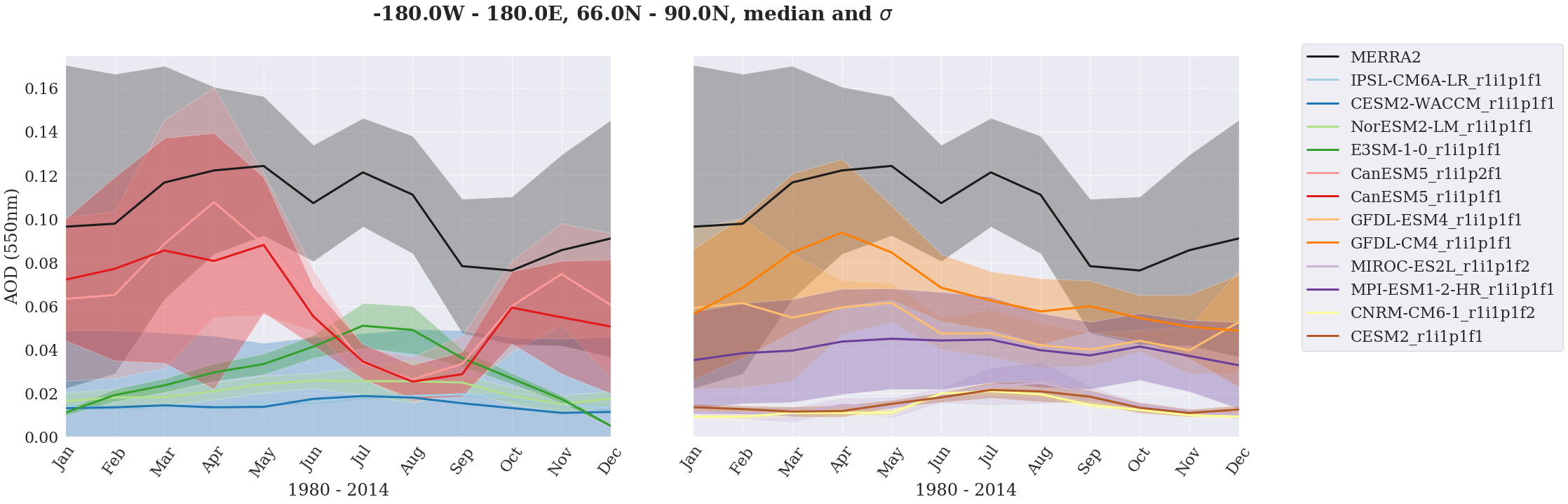
Fig. 3 shows the monthly median averages for AOD in the Arctic region between 1980-2014. The black line indicates the MERRA2 reanalysis with its variability in grey shading. As expected, is the MERRA2 variability of AOD largest in the Arctic winter during the polar night. Since AOD is measured optically it is not possible for the satellites (MODIS) to retrieve the AOD at 550nm during Arctic winter due to the lack of light. It also has to be taken into account, that AOD cannot be retrieved for cloudy days cloudy grid cells, and over snow/ice ground for MERRA2. Perhaps the MERRA2 values were interpolated from other wavelength retrieved by different satellites during winter.
We see in Fig. 2 a seasonal variation of AOD at the stations and for MERRA2 data. In Fig. 3 the MERRA2 reanalysis shows a peak of AOD during spring and summer and is for a longer average consistent with the seasonal cycle presented in Fig. 2. Here again, Arctic haze during spring, biogas burning and volcanic eruption come into play over the 1980 to 2014 period.
The coloured lines show the AOD from the CMIP6 model medians and their variability for the 34-year average. None of the here evaluated CMIP6 models simulates the AOD values during the summer month (June - August).
One CMIP6 model, namely, CanESM5 (red) catches one's eye. It simulates a distinct peak of AOD with large variability overlapping the MERRA2 reanalysis during Arctic spring for the 1980 - 2014 averages. On the other hand, the CanESM5 is too low during summer and not within the MERRA2 variability. A reason for the good simulation during spring can be an enhancement due to continental aerosols from midlatitudes and a higher amount of marine aerosols, driven by surface winds. The GFDL-ESM4 model (orange) is within the MERRA2 variability in the winter month until spring (September – March), but again too low during summer.
Glantz et al., 2014 studied the previous version of NorESM2-LM by validating it with MODIS satellite AOD measurements. The NorESM1-M CMIP5 model showed then too low values for AOD at 550nm. In Fig. 3 we can see that NorESM-LM (light green) is almost constant over the year. E3SM-1-0, on the other hand, shows the best estimate of summer AOD, although too low compared to the measurements.
# Figure 4
starty = '1980'; endy = '2014'
fig, ax = plt.subplots(1, figsize=[20,7])
(merra_zonal['median_'+starty+endy] - merra_zonal['M2IMNXGAS_5_12_4_AODANA'].sel(time=slice(starty+'-01',endy+'-12')) ).plot(ax=ax,
                                                                                                             cmap= plt.get_cmap('RdGy'),
                                                                                                             vmin=-0.1,vmax=0.1,extend='both',
                                                                                                             robust=True,
                                                                                                             cbar_kwargs={"ticks": np.arange(-0.1,0.15,0.05),
                                                                                                                         "label": "$\Delta$AOD (550nm)"})
xlabels = ['1980', '1982', '1984' ,'1986', '1988',
           '1990', '1992', '1994' ,'1996', '1998',
           '2000', '2002', '2004' ,'2006', '2008',
           '2010', '2012', '2014' ,]
ax.set_xlabel('Years')
ax.set_xlim(['1980-01-01', '2015-01-01'])
ax.set_xticks(xlabels)
ax.set_xticklabels(xlabels,rotation=80)
ax.set_ylabel('Latitude (deg)')
ax.set_ylim([-90,90])
ax.set_yticks(np.arange(-90,120,30))
ax.axvline('1990-01-01', linewidth=3, color='k')
ax.axvline('2000-01-01', linewidth=3, color='k')
ax.axvline('2009-12-31', linewidth=3, color='k')
ax.set_title('1980-2014 - AOD$_{year}$');

if savefig == 1:
    filename = './Figures/Hovemoeller_MERRA2.png'
    plt.savefig(filename,#transparent=True,
                bbox_inches='tight');
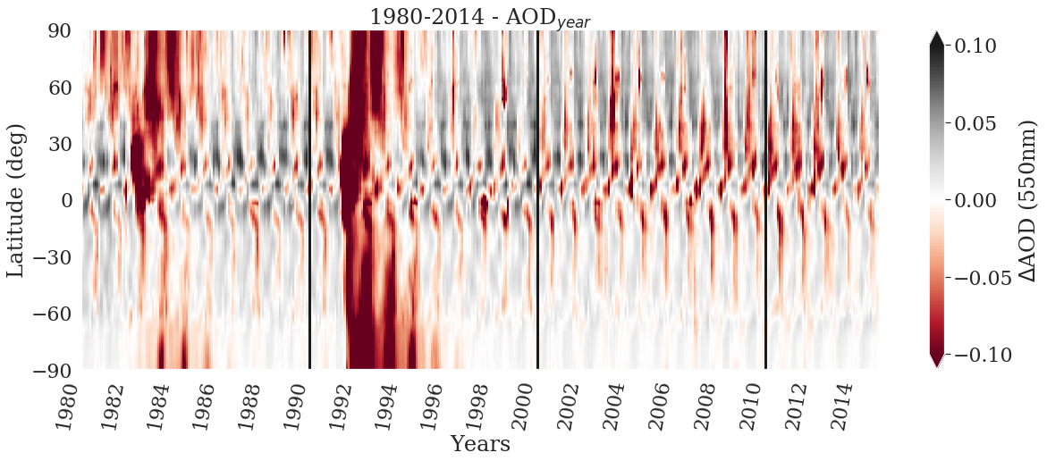
The alteration of zonally averaged AOD compared to the 1980 - 2014 climatology shows in Fig. 4. Red shading represents an AOD increase. An AOD increase is globally distinct after the Mount Pinatubo eruption in June 1991 and consists for three years after. Generally shows Fig. 4 a seasonal pattern with an AOD decrease in the tropics during winter and an increase during summer.
The winter months show a stronger decrease (red) of AOD in the Northern Hemispheric tropical zone (~up to 30$^\circ$N) when comparing the 2000s and 2010s to the late 1980s. On the other hand, the summer months show a stronger decrease of AOD in the mid- and high latitudes of the Northern Hemisphere. Increased production of anthropogenic aerosols leads to a decrease of AOD in the Northern Hemisphere since the 2000s.
# Figure 5
fig, axsm = plt.subplots(4,4, sharex = 'all', sharey='all',
                         figsize=[28,20])
axs = axsm.flatten()
starty ='1980'; endy='2014'

# Plot MERRA median in each plot of the model
for i in range(4,len(_mm)+4):
    merra_zonal['median_'+starty+endy].plot(ax = axs[i], linewidth=3, color='k',
                                  label='MERRA2 (%s-%s)' %(starty,endy))
    axs[i].fill_between(merra_zonal['median_'+starty+endy].lat,
                           merra_zonal['median_'+starty+endy] - merra_zonal['std_'+starty+endy],
                           merra_zonal['median_'+starty+endy] + merra_zonal['std_'+starty+endy],
                           alpha=0.3, facecolor='k')
# Plot each decade in the subplots for MERRA and the CMIP models
for yr, l_style in zip(['19801989', '19901999', '20002009'], ['-', ':', '-.']):
    merra_zonal['median_'+yr].plot(ax=axs[0], linewidth=4, linestyle = l_style)
    axs[0].fill_between(merra_zonal['median_'+yr].lat,
                        merra_zonal['median_'+yr] - merra_zonal['std_'+yr],
                        merra_zonal['median_'+yr] + merra_zonal['std_'+yr],
                        alpha=0.3)

    for model, rea, i in zip(_mm, _rr, range(4,len(_mm)+4)):

        fct.plt_zonal_model_merra(axs[i], cmip[model][rea]['median_'+yr],
                              cmip[model][rea]['std_'+yr],
                                  merra_zonal['median_'+starty+endy], merra_zonal['std_'+starty+endy],
                                  model, sns.color_palette("Paired",12)[i-4])
        axs[i].set_title('%s' %model, fontweight='bold')


axs[0].set_title('MERRA2', fontweight='bold')
axs[0].legend(['1980 - 1989','1990 - 1999', '2000 - 2009'],bbox_to_anchor=(1.1, 1.05))# loc='center right')
axs[4].legend()
for i in range(1,4):
    axs[i].set_visible(False)

for i in np.arange(0,16,4):
    axs[i].set_ylabel('AOD (550nm)')
for i, j, k in zip(np.arange(5,9), np.arange(9,13), np.arange(13,16)):
    axs[i].set_ylabel('')
    axs[j].set_ylabel('')
    axs[k].set_ylabel('')
for i in range(0,12):
    axs[i].set_xlabel('')
for i in range(12,16):
    axs[i].set_xlabel('Latitude (deg)')
    axs[i].set_xlim([-90,90])
    axs[i].set_xticks(np.arange(-90,120,30))

plt.subplots_adjust(wspace = 0.2,
                    hspace = 0.2   );
if savefig == 1:
    filename = './Figures/zonal_CMIP6.png'
    plt.savefig(filename,#transparent=True,
                bbox_inches='tight');
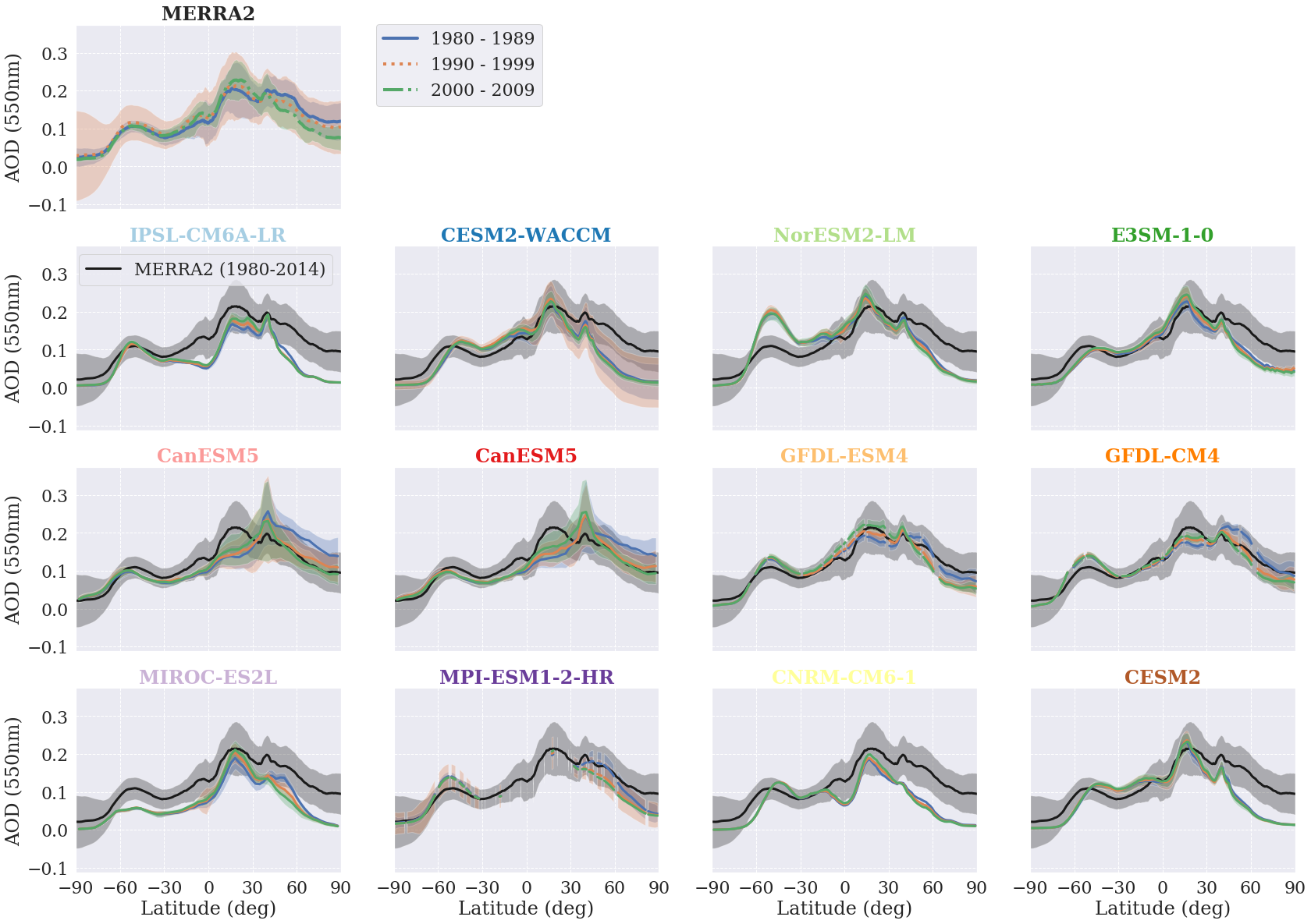
Fig. 5 upper panel shows the MERRA2 zonally averaged AOD for three decades, the 1980s, 1990s and 2000s. Around 60$^\circ$S we see the AOD dominated by sea salt, in the Tropics (15$^\circ$N) the influence by Saharan dust and the midlatitudes in the Northern Hemisphere influence by biogas burning and anthropogenic emissions. Especially in the Northern Hemisphere, we see a decrease of AOD in the mid- and higher latitudes (compare the 1980s to 2000s). Fig. 5 second to the fourth row shows the MERRA2 zonally averaged AOD trend calculated for 1980-2014 and the CMIP6 models used in this study. In most of the CMIP6 models, we see no difference between the three decades. Only CanESM5, GFDL-ESM4, GFDL-CM4, MIROC-ES2L and MPI-ESM1-2-HR show higher AOD for the 1980s above 30$^\circ$N (blue line).
Most of the here studied CMIP6 models underestimate the AOD in the mid- and high latitudes of the Northern Hemisphere, as already seen in the seasonal variation of the Arctic averaged AOD (Fig. 3). The CMIP6 GFDL models simulate the best zonal averaged AOD. The zonal average fits the variation of MERRA2 trend and is within the uncertainty of the reanalysis.
Most of the models have a small uncertainty for the three decades. CESM2-WACCM shows the largest variability compared to all CMIP6 models, especially in the Northern Hemisphere in the 1990s. The high variability might be associated with the volcanic forcing of the model during the Pinatubo eruption in 1991. NorESM-LM does partly not follow the zonal trend reanalysed by MERRA2. NorESM-LM has high AOD values in the Southern Hemisphere. On the other hand, the AOD in the Northern Hemisphere above 40$^\circ$N is not within the uncertainty of the MERRA2 reanalysis and valid for all three decades. Sofie Tunes compares the relation between sea salt and wind at Ny Ålesund and the Zeppelin Station (Svalbard). Her work shows higher values of sea salt in NorESM2-LM for this specific location. The question arises, if NorESM2-LM produces too much sea salt why is the AOD in the Arctic too low and almost does not show a seasonal variation of AOD in Fig. 3. Too much sea salt would mean more possible cloud condensation nuclei (CCN) will exist. Hence liquid water will be distributed equally over a larger number of CCNs. The cloud is then made up of smaller cloud droplets and will have a higher optical depth than clouds with fewer cloud droplets. Clouds with high optical depth will reflect more incoming radiation and could, therefore, have a cooling effect on the earth system (Lamb and Verlinde, 2011). But further studies should be carried out to find the reason for the high sea salt around 60$^\circ$S and on the other hand too little AOD in the Arctic. CanESM5 shows in Fig. 3 a good agreement of AOD peak during the Arctic spring. CanESM5 simulates too low zonal averaged AOD in the tropics and subtropics and too high AOD in midlatitudes of the Northern Hemisphere. Compared to MERRA2, CanESM5 has a shifted AOD peak, instead of 15$^\circ$N at 40$^\circ$N. It agrees with the decadal trend seen with MERRA2, namely a decrease of AOD in the Northern Hemisphere (panel MERRA2 and CanESM5). The CMIP6 models MIROC-ES2L and CNRM-CM6-1 simulate almost no seasonal cycle for the Arctic in Fig. 3. Both these models underestimate the zonal AOD nearly everywhere. Too little aerosols mean more sunlight can reach the ground and hence, the global surface temperature increases.
Summary and Conclusion
In this project, I analysed how representative the MERRA2 satellite reanalysis is in comparison to the ground-based AOD Sunphotometers for Arctic stations. We used this further to see how representative a fine-scale Arctic average of MERRA2 reanalysis can be. The MERRA2 reanalysis helped us to do a seasonal intercomparison of 12 CMIP6 models for the Arctic region during 1980 - 2014. We analysed the CMIP6 models to the decadal change of zonally averaged AOD since 1980. MERRA2 reanalysis is barely within the variability of the AERONET Sunphotometer observations and generally overestimates compared to the stations. Seasonal variation of Arctic AOD was reanalysed by MERRA2 with higher values during Arctic spring and summer. Sunphotometer observations are barely within the MERRA2 uncertainty, and further analysis has to be done to understand the higher values of MERRA2.
In average, the largest variability of AOD reanalysed by MERRA2 was seen during Arctic winter. The seasonal variation for monthly AOD average was mainly not reproduced by the CMIP6 models, as already seen for the CMIP5 models (Glantz et al., 2014). CanESM5 is within the range of MERRA2 during spring but on the other side too low in the summertime. GFDL-ESM4 is within the MERRA2 variability during winter and has a weak seasonal pattern. NorESM-LM shows a weak seasonal variation of AOD in the Arctic with the highest values during summer. E3SM-1-0 simulates the AOD during summer but is in general too weak compared to MERRA2 reanalysis.
The GFDL-ESM4 and GFDL-CM4 model fit zonally the best for all three decades.
CESM2-WACCM had the highest variability in the Northern Hemisphere, especially the Arctic for all three decades.
NorESM2-LM does not reproduce the AOD zonal averages as reanalysed by MERRA2. It produces too high sea salt in the Southern Hemisphere and too little AOD above 60$^\circ$N.
CanESM5 reproduces the AOD pattern along the latitude, but the AOD peak in the Northern subtropics is shifted towards North with no peak in the tropics (Saharan dust) and too high AOD in the subtropics (human emissions and biogas burning).
The two CMIP6 models MIROC-ES2L and CNRM-CM6-1 have too low AOD values zonally compared to the MERRA2 reanalysis.
A continuation of this work can be to analyse the different aerosol compounds in the vertical and how they differ between the CMIP6 models. Furthermore, an in-depth study of NorESM-LM should be implemented to find the reason for the high sea salt in the Southern Hemisphere and the low AOD in the Arctic. The MERRA2 reanalysis has to be more understood, especially how winter AOD is retrieved at high latitudes.
Acknowledgement
I would like to thank our group assistants Ksenia, and Paul who helped me with the MERRA2 data and the topic, and Jonas who made pyaerocom understandable. All the other assistants and teachers were also very helpful in particular, Sara who helped me with xarray and making my code more efficient. Thanks to Eemeli for helpful comments on my report. Thanks to Anne for all the help on Jupyterhub and Github.
I also want to thank the CHESS research school on changing climates in the coupled earth system which made it possible to attend the course in Abisko.
This study was performed on Jupyterhub on resources provided by UNINETT Sigma2 - the National Infrastructure for High-Performance Computing and Data Storage in Norway as part of NS1000K project. Data was downloaded through NASAs GIOVANNI interface.
References
Collins, M., Knutti, R., Arblaster, J., Dufresne, J.-L., Fichefet, T., Friedlingstein, P., Gao, X., Gutowski, W.J., Johns, T., Krinner, G., Shongwe, M., Tebaldi, C., Weaver, A.J., Wehner, M., 2013. Long-term Climate Change: Projections, Commitments and Irreversibility, in: Stocker, T.F., Qin, D., Plattner, G.-K., Tignor, M., Allen, S.K., Boschung, J., Nauels, A., Xia, Y., Bex, V., Midgley, P.M. (Eds.), Climate Change 2013: The Physical Science Basis. Contribution of Working Group I to the Fifth Assessment Report of the Intergovernmental Panel on Climate Change. Cambridge University Press, Cambridge, United Kingdom and New York, NY, USA, pp. 1029–1136. https://doi.org/10.1017/CBO9781107415324.024
Eyring, V., Bony, S., Meehl, G.A., Senior, C.A., Stevens, B., Stouffer, R.J., Taylor, K.E., 2016. Overview of the Coupled Model Intercomparison Project Phase 6 (CMIP6) experimental design and organization. Geosci. Model Dev. 9, 1937–1958. https://doi.org/10.5194/gmd-9-1937-2016
Gelaro, R., McCarty, W., Suárez, M.J., Todling, R., Molod, A., Takacs, L., Randles, C.A., Darmenov, A., Bosilovich, M.G., Reichle, R., Wargan, K., Coy, L., Cullather, R., Draper, C., Akella, S., Buchard, V., Conaty, A., da Silva, A.M., Gu, W., Kim, G.-K., Koster, R., Lucchesi, R., Merkova, D., Nielsen, J.E., Partyka, G., Pawson, S., Putman, W., Rienecker, M., Schubert, S.D., Sienkiewicz, M., Zhao, B., 2017. The Modern-Era Retrospective Analysis for Research and Applications, Version 2 (MERRA-2). J. Climate 30, 5419–5454. https://doi.org/10.1175/JCLI-D-16-0758.1
Giles, D.M., Sinyuk, A., Sorokin, M.G., Schafer, J.S., Smirnov, A., Slutsker, I., Eck, T.F., Holben, B.N., Lewis, J.R., Campbell, J.R., Welton, E.J., Korkin, S.V., Lyapustin, A.I., 2019. Advancements in the Aerosol Robotic Network (AERONET) Version 3 database – automated near-real-time quality control algorithm with improved cloud screening for Sun photometer aerosol optical depth (AOD) measurements. Atmospheric Measurement Techniques 12, 169–209. https://doi.org/10.5194/amt-12-169-2019
Glantz, P., Bourassa, A., Herber, A., Iversen, T., Karlsson, J., Kirkevåg, A., Maturilli, M., Seland, Ø., Stebel, K., Struthers, H., Tesche, M., Thomason, L., 2014. Remote sensing of aerosols in the Arctic for an evaluation of global climate model simulations. Journal of Geophysical Research: Atmospheres 119, 8169–8188. https://doi.org/10.1002/2013JD021279
Golaz, J.-C., Caldwell, P.M., Roekel, L.P.V., Petersen, M.R., Tang, Q., Wolfe, J.D., Abeshu, G., Anantharaj, V., Asay‐Davis, X.S., Bader, D.C., Baldwin, S.A., Bisht, G., Bogenschutz, P.A., Branstetter, M., Brunke, M.A., Brus, S.R., Burrows, S.M., Cameron‐Smith, P.J., Donahue, A.S., Deakin, M., Easter, R.C., Evans, K.J., Feng, Y., Flanner, M., Foucar, J.G., Fyke, J.G., Griffin, B.M., Hannay, C., Harrop, B.E., Hoffman, M.J., Hunke, E.C., Jacob, R.L., Jacobsen, D.W., Jeffery, N., Jones, P.W., Keen, N.D., Klein, S.A., Larson, V.E., Leung, L.R., Li, H.-Y., Lin, W., Lipscomb, W.H., Ma, P.-L., Mahajan, S., Maltrud, M.E., Mametjanov, A., McClean, J.L., McCoy, R.B., Neale, R.B., Price, S.F., Qian, Y., Rasch, P.J., Eyre, J.E.J.R., Riley, W.J., Ringler, T.D., Roberts, A.F., Roesler, E.L., Salinger, A.G., Shaheen, Z., Shi, X., Singh, B., Tang, J., Taylor, M.A., Thornton, P.E., Turner, A.K., Veneziani, M., Wan, H., Wang, H., Wang, S., Williams, D.N., Wolfram, P.J., Worley, P.H., Xie, S., Yang, Y., Yoon, J.-H., Zelinka, M.D., Zender, C.S., Zeng, X., Zhang, C., Zhang, K., Zhang, Y., Zheng, X., Zhou, T., Zhu, Q., 2019. The DOE E3SM Coupled Model Version 1: Overview and Evaluation at Standard Resolution. Journal of Advances in Modeling Earth Systems 11, 2089–2129. https://doi.org/10.1029/2018MS001603
Hajima, T., Watanabe, M., Yamamoto, A., Tatebe, H., Noguchi, M.A., Abe, M., Ohgaito, R., Ito, Akinori, Yamazaki, D., Okajima, H., Ito, Akihiko, Takata, K., Ogochi, K., Watanabe, S., Kawamiya, M., 2019. Description of the MIROC-ES2L Earth system model and evaluation of its climate–biogeochemical processes and feedbacks. Geoscientific Model Development Discussions 1–73. https://doi.org/10.5194/gmd-2019-275
Held, I.M., Guo, H., Adcroft, A., Dunne, J.P., Horowitz, L.W., Krasting, J., Shevliakova, E., Winton, M., Zhao, M., Bushuk, M., Wittenberg, A.T., Wyman, B., Xiang, B., Zhang, R., Anderson, W., Balaji, V., Donner, L., Dunne, K., Durachta, J., Gauthier, P.P.G., Ginoux, P., Golaz, J.-C., Griffies, S.M., Hallberg, R., Harris, L., Harrison, M., Hurlin, W., John, J., Lin, P., Lin, S.-J., Malyshev, S., Menzel, R., Milly, P.C.D., Ming, Y., Naik, V., Paynter, D., Paulot, F., Ramaswamy, V., Reichl, B., Robinson, T., Rosati, A., Seman, C., Silvers, L., Underwood, S., Zadeh, N., 2019. Structure and Performance of GFDL’s CM4.0 Climate Model. Journal of Advances in Modeling Earth Systems 0. https://doi.org/10.1029/2019MS001829
Kirkevåg, A., Grini, A., Olivié, D., Seland, Ø., Alterskjær, K., Hummel, M., Karset, I.H.H., Lewinschal, A., Liu, X., Makkonen, R., Bethke, I., Griesfeller, J., Schulz, M., Iversen, T., 2018. A production-tagged aerosol module for Earth system models, OsloAero5.3 – extensions and updates for CAM5.3-Oslo. Geosci. Model Dev. 11, 3945–3982. https://doi.org/10.5194/gmd-11-3945-2018
Lamb, D., Verlinde, J., 2011. Physics and Chemistry of Clouds. Cambridge University Press, Cambridge. https://doi.org/10.1017/CBO9780511976377
Lohmann, U., Luond, F., Mahrt, F., 2016. An Introduction to Clouds: From the Microscale to Climate. Cambridge University Press, Cambridge. https://doi.org/10.1017/CBO9781139087513
NCAR CESM2, 2018. NCAR CESM2 model output prepared for CMIP6. Earth System Grid Federation. https://doi.org/10.5065/D67H1H0V
Swart, N.C., Cole, J.N.S., Kharin, V.V., Lazare, M., Scinocca, J.F., Gillett, N.P., Anstey, J., Arora, V., Christian, J.R., Hanna, S., Jiao, Y., Lee, W.G., Majaess, F., Saenko, O.A., Seiler, C., Seinen, C., Shao, A., Solheim, L., Salzen, K. von, Yang, D., Winter, B., 2019. The Canadian Earth System Model version 5 (CanESM5.0.3). Geoscientific Model Development Discussions 1–68. https://doi.org/10.5194/gmd-2019-177
Voldoire, A., Saint‐Martin, D., Sénési, S., Decharme, B., Alias, A., Chevallier, M., Colin, J., Guérémy, J.-F., Michou, M., Moine, M.-P., Nabat, P., Roehrig, R., Mélia, D.S. y, Séférian, R., Valcke, S., Beau, I., Belamari, S., Berthet, S., Cassou, C., Cattiaux, J., Deshayes, J., Douville, H., Ethé, C., Franchistéguy, L., Geoffroy, O., Lévy, C., Madec, G., Meurdesoif, Y., Msadek, R., Ribes, A., Sanchez‐Gomez, E., Terray, L., Waldman, R., 2019. Evaluation of CMIP6 DECK Experiments With CNRM-CM6-1. Journal of Advances in Modeling Earth Systems 11, 2177–2213. https://doi.org/10.1029/2019MS001683
!jupyter nbconvert --to html franzihe_area_averaged_AOD_V2.ipynb
!jupyter nbconvert --to pdf franzihe_area_averaged_AOD_V2.ipynb
!jupyter nbconvert --to markdown franzihe_area_averaged_AOD_V2.ipynb
#!jupyter nbconvert --to html --template ./clean_output.tpl franzihe_area_averaged_AOD_V2.ipynb