.ipynb .pdf

repository open issue

Binder

Contents

Using pydap and pandas to read EBAS data

See more at http://ebas.nilu.no/

The EBAS database collects observational data on atmospheric chemical composition and physical properties from a variety of national and international research projects and monitoring programs, such as ACTRIS, AMAP, EMEP, GAW and HELCOM, as well as for the Norwegian monitoring programs funded by the Norwegian Environment Agency, the Ministry of Climate and Environment and NILU – Norwegian Institute for Air Research.

Import Python packages

from pydap.client import open_dods, open_url
from netCDF4 import num2date
import pandas as pd
import cftime
import matplotlib.pyplot as plt

Get data directly from EBAS database

• syntax: ST_STATION_CODE.FT_TYPE.RE_REGIME_CODE.MA_MATRIX_NAME.CO_COMP_NAME.DS_RESCODE.FI_REF.ME_REF.DL_DATA_LEVEL.dods

• or: #station.instrument_type.IMG.matrix.component.resolution.instrument_reference.datalevel.dods

• if no level, then ..dods

• if doesn’t work, download one file to check what are the FI_REF and ME_REF.

• other example: http://dev-ebas-pydap.nilu.no/NO0042G.Hg_mon.IMG.air.mercury.1h.NO01L_tekran_42_dup.NO01L_afs..dods

# get directly from EBAS
ds = open_dods(
'http://dev-ebas-pydap.nilu.no/' 
'NO0042G.dmps.IMG.aerosol.particle_number_size_distribution'
'.1h.NO01L_NILU_DMPSmodel2_ZEP.NO01L_dmps_DMPS_ZEP01.2.dods')

Format data into pandas dataframe

#get the actual data
dmps_data = ds['particle_number_size_distribution_amean']

# get normalised size distribution in dNdlogDp
dNdlogDp = dmps_data.particle_number_size_distribution_amean.data

# get time in datatime format using function from netCDF4 package
tim_dmps = num2date(dmps_data.time.data,units='days since 1900-01-01 00:00:00',
calendar ='gregorian')

# get diameter vector
dp_NILU = dmps_data.D.data

# make DataFrame to simplify the handling of data
df_NILU = pd.DataFrame(dNdlogDp.byteswap().newbyteorder(), index=dp_NILU, columns=tim_dmps)

df_NILU.head()

	2016-05-06 05:30:00	2016-05-06 06:30:00	2016-05-06 07:30:00	2016-05-06 08:30:00	2016-05-06 09:30:00	2016-05-06 10:30:00	2016-05-06 11:30:00	2016-05-06 12:30:00	2016-05-06 13:30:00	2016-05-06 14:30:00	...	2017-12-31 14:30:00	2017-12-31 15:30:00	2017-12-31 16:30:00	2017-12-31 17:30:00	2017-12-31 18:30:00	2017-12-31 19:30:00	2017-12-31 20:30:00	2017-12-31 21:30:00	2017-12-31 22:30:00	2017-12-31 23:30:00
10.0	20.16	27.86	33.89	38.96	32.82	44.25	295.19	697.74	840.26	946.78	...	8.52	8.29	13.86	8.18	9.96	8.41	6.92	9.81	10.94	6.79
12.0	41.16	37.93	46.07	53.32	50.76	66.31	169.43	543.82	1132.41	1570.59	...	8.50	9.41	7.67	7.36	6.70	7.47	7.53	7.19	6.92	7.05
14.0	59.79	48.38	57.63	64.44	68.81	92.40	100.44	330.05	889.54	1576.16	...	10.86	11.29	5.13	8.20	5.69	6.98	8.08	5.97	4.80	10.96
17.0	52.01	45.14	56.40	62.01	73.59	102.47	79.43	117.88	266.77	772.37	...	15.88	13.76	8.77	9.54	8.48	7.13	7.99	6.12	5.17	12.47
21.0	21.98	28.03	37.41	44.52	54.98	73.01	87.58	115.21	152.36	243.23	...	23.46	17.98	23.14	11.82	15.61	9.80	8.35	9.21	8.28	7.09

5 rows × 14515 columns

Select time and Plot

df_NILU.columns

Index([2016-05-06 05:30:00, 2016-05-06 06:30:00, 2016-05-06 07:30:00,
       2016-05-06 08:30:00, 2016-05-06 09:30:00, 2016-05-06 10:30:00,
       2016-05-06 11:30:00, 2016-05-06 12:30:00, 2016-05-06 13:30:00,
       2016-05-06 14:30:00,
       ...
       2017-12-31 14:30:00, 2017-12-31 15:30:00, 2017-12-31 16:30:00,
       2017-12-31 17:30:00, 2017-12-31 18:30:00, 2017-12-31 19:30:00,
       2017-12-31 20:30:00, 2017-12-31 21:30:00, 2017-12-31 22:30:00,
       2017-12-31 23:30:00],
      dtype='object', length=14515)

type(df_NILU.columns[0])

cftime._cftime.DatetimeGregorian

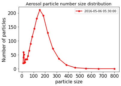
tsel = cftime.DatetimeGregorian(2016, 5, 6, 5, 30)

fig = plt.figure(1, figsize=[15,5])
ax = df_NILU[tsel].plot(lw=2, colormap='coolwarm', marker='.', markersize=10, title='Aerosol particle number size distribution', fontsize=15)
ax.set_xlabel("particle size", fontsize=15)
ax.set_ylabel("Number of particles", fontsize=15)
ax.title.set_size(20)

Save into a local csv file

filename = 'size_dist' + tsel.strftime('%d%B%Y_%H%M') + '.csv'
print(filename)

size_dist06May2016_0530.csv

df_NILU[tsel].to_csv(filename, sep='\t', index=True, header=True)

Save into Galaxy history

• You can also use bioblend python package to directly interact with your galaxy history

!put -p size_dist06May2016_0530.csv -t tabular

Save to NIRD via s3fs

• Make sure you have your credential in $HOME/.aws/credentials

import s3fs

Set the path on NIRD (and add “s3:/” in front of it)

s3_path = "s3://work/" + filename
print(s3_path)

s3://work/size_dist06May2016_0530.csv

fsg = s3fs.S3FileSystem(anon=False,
      client_kwargs={
         'endpoint_url': 'https://forces2021.uiogeo-apps.sigma2.no/'
      })

bytes_to_write = df_NILU[tsel].to_csv(None, sep='\t', index=True, header=True).encode()

with fsg.open(s3_path, 'wb') as f:
    f.write(bytes_to_write)

Check your file

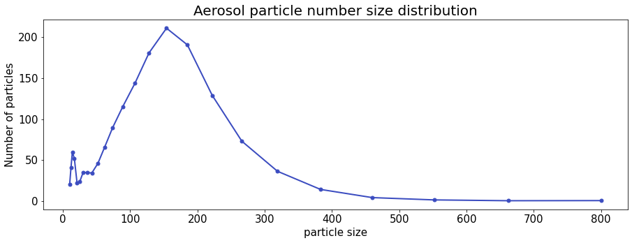
dfo = pd.read_csv(fsg.open(s3_path), sep='\t', index_col=0)

dfo.head()

	2016-05-06 05:30:00
10.0	20.16
12.0	41.16
14.0	59.79
17.0	52.01
21.0	21.98

ax = dfo.plot(lw=2, color='red', marker='.', markersize=10, title='Aerosol particle number size distribution', fontsize=15)
ax.set_xlabel("particle size", fontsize=15)
ax.set_ylabel("Number of particles", fontsize=15)
ax.title.set_size(14)

previous

Using ADAM-API to access UERRA regional reanalysis

next

Using xarray to read EBAS data