.ipynb .pdf

repository open issue

Binder

Contents

Multidimensional Coordinates example using CMIP6 Pangeo ocean model data

Import python packages

import xarray as xr
xr.set_options(display_style='html')
import intake
import cftime
import matplotlib.pyplot as plt
import matplotlib.path as mpath
import cartopy.crs as ccrs
import numpy as np
%matplotlib inline

Open CMIP6 online catalog

cat_url = "https://storage.googleapis.com/cmip6/pangeo-cmip6.json"
col = intake.open_esm_datastore(cat_url)
col

pangeo-cmip6 catalog with 7715 dataset(s) from 520279 asset(s):

	unique
activity_id	18
institution_id	36
source_id	88
experiment_id	170
member_id	657
table_id	37
variable_id	709
grid_label	10
zstore	520279
dcpp_init_year	60
version	723

Search corresponding data

cat = col.search(source_id=['MPI-ESM1-2-HR'], experiment_id=['historical'], table_id=['Omon'], variable_id=['chl'], member_id=['r9i1p1f1'])
cat.df

	activity_id	institution_id	source_id	experiment_id	member_id	table_id	variable_id	grid_label	zstore	dcpp_init_year	version
0	CMIP	MPI-M	MPI-ESM1-2-HR	historical	r9i1p1f1	Omon	chl	gn	gs://cmip6/CMIP6/CMIP/MPI-M/MPI-ESM1-2-HR/hist...	NaN	20190710

Create dictionary from the list of datasets we found

• This step may take several minutes so be patient!

dset_dict = cat.to_dataset_dict(zarr_kwargs={'use_cftime':True})

--> The keys in the returned dictionary of datasets are constructed as follows:
	'activity_id.institution_id.source_id.experiment_id.table_id.grid_label'

100.00% [1/1 00:00<00:00]

list(dset_dict.keys())

['CMIP.MPI-M.MPI-ESM1-2-HR.historical.Omon.gn']

Open dataset

• Use xarray python package to analyze netCDF dataset

• open_dataset allows to get all the metadata without loading data into memory.

• with xarray, we only load into memory what is needed.

dset = dset_dict['CMIP.MPI-M.MPI-ESM1-2-HR.historical.Omon.gn']
dset

<xarray.Dataset>
Dimensions:             (bnds: 2, i: 802, j: 404, lev: 40, member_id: 1, time: 1980, vertices: 4)
Coordinates:
  * i                   (i) int32 0 1 2 3 4 5 6 ... 795 796 797 798 799 800 801
  * j                   (j) int32 0 1 2 3 4 5 6 ... 397 398 399 400 401 402 403
    latitude            (j, i) float64 dask.array<chunksize=(404, 802), meta=np.ndarray>
  * lev                 (lev) float64 6.0 17.0 27.0 ... 5.17e+03 5.72e+03
    lev_bnds            (lev, bnds) float64 dask.array<chunksize=(40, 2), meta=np.ndarray>
    longitude           (j, i) float64 dask.array<chunksize=(404, 802), meta=np.ndarray>
  * time                (time) object 1850-01-16 12:00:00 ... 2014-12-16 12:0...
    time_bnds           (time, bnds) object dask.array<chunksize=(1980, 2), meta=np.ndarray>
  * member_id           (member_id) <U8 'r9i1p1f1'
Dimensions without coordinates: bnds, vertices
Data variables:
    chl                 (member_id, time, lev, j, i) float32 dask.array<chunksize=(1, 2, 40, 404, 802), meta=np.ndarray>
    vertices_latitude   (j, i, vertices) float64 dask.array<chunksize=(404, 802, 4), meta=np.ndarray>
    vertices_longitude  (j, i, vertices) float64 dask.array<chunksize=(404, 802, 4), meta=np.ndarray>
Attributes: (12/50)
    Conventions:             CF-1.7 CMIP-6.2
    activity_id:             CMIP
    branch_method:           standard
    branch_time_in_child:    0.0
    branch_time_in_parent:   146096.0
    cmor_version:            3.5.0
    ...                      ...
    title:                   MPI-ESM1-2-HR output prepared for CMIP6
    tracking_id:             hdl:21.14100/4e922d88-7711-4df6-9bdd-b849acd45a7...
    variable_id:             chl
    variant_label:           r9i1p1f1
    intake_esm_varname:      ['chl']
    intake_esm_dataset_key:  CMIP.MPI-M.MPI-ESM1-2-HR.historical.Omon.gn

Get metadata corresponding to Chl

print(dset['chl'])

<xarray.DataArray 'chl' (member_id: 1, time: 1980, lev: 40, j: 404, i: 802)>
dask.array<broadcast_to, shape=(1, 1980, 40, 404, 802), dtype=float32, chunksize=(1, 2, 40, 404, 802), chunktype=numpy.ndarray>
Coordinates:
  * i          (i) int32 0 1 2 3 4 5 6 7 8 ... 794 795 796 797 798 799 800 801
  * j          (j) int32 0 1 2 3 4 5 6 7 8 ... 396 397 398 399 400 401 402 403
    latitude   (j, i) float64 dask.array<chunksize=(404, 802), meta=np.ndarray>
  * lev        (lev) float64 6.0 17.0 27.0 37.0 ... 4.67e+03 5.17e+03 5.72e+03
    longitude  (j, i) float64 dask.array<chunksize=(404, 802), meta=np.ndarray>
  * time       (time) object 1850-01-16 12:00:00 ... 2014-12-16 12:00:00
  * member_id  (member_id) <U8 'r9i1p1f1'
Attributes:
    cell_measures:  area: areacello volume: volcello
    cell_methods:   area: mean where sea time: mean
    comment:        Sum of chlorophyll from all phytoplankton group concentra...
    history:        2019-08-30T07:10:19Z altered by CMOR: replaced missing va...
    long_name:      Mass Concentration of Total Phytoplankton Expressed as Ch...
    original_name:  chl
    standard_name:  mass_concentration_of_phytoplankton_expressed_as_chloroph...
    units:          kg m-3

dset.time.values

array([cftime.DatetimeProlepticGregorian(1850, 1, 16, 12, 0, 0, 0),
       cftime.DatetimeProlepticGregorian(1850, 2, 15, 0, 0, 0, 0),
       cftime.DatetimeProlepticGregorian(1850, 3, 16, 12, 0, 0, 0), ...,
       cftime.DatetimeProlepticGregorian(2014, 10, 16, 12, 0, 0, 0),
       cftime.DatetimeProlepticGregorian(2014, 11, 16, 0, 0, 0, 0),
       cftime.DatetimeProlepticGregorian(2014, 12, 16, 12, 0, 0, 0)],
      dtype=object)

Visualization

shift longitude from 0,360 to -180,180

dset.coords['longitude'] = (dset['longitude'] + 180) % 360 - 180

dset['chl'].latitude.values.min(), dset['chl'].latitude.values.max()

(-78.71779338013427, 89.76311914726304)

dset['chl'].longitude.values.min(), dset['chl'].longitude.values.max()

(-179.99408443971072, 179.99893486577713)

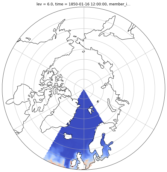
Select geographical area, time and level

dset_selection = dset.isel(time=0, lev=0).where( (dset.latitude > 50) & (dset.longitude > -30) & (dset.longitude < 30) ).squeeze()

def polarCentral_set_latlim(lat_lims, ax):
    ax.set_extent([-180, 180, lat_lims[0], lat_lims[1]], ccrs.PlateCarree())
    # Compute a circle in axes coordinates, which we can use as a boundary
    # for the map. We can pan/zoom as much as we like - the boundary will be
    # permanently circular.
    theta = np.linspace(0, 2*np.pi, 100)
    center, radius = [0.5, 0.5], 0.5
    verts = np.vstack([np.sin(theta), np.cos(theta)]).T
    circle = mpath.Path(verts * radius + center)

    ax.set_boundary(circle, transform=ax.transAxes)

fig = plt.figure(1, figsize=[10,10])

# Fix extent
minval = 0
maxval = 100.

ax = plt.subplot(1, 1, 1, projection=ccrs.NorthPolarStereo())
ax.coastlines()
ax.gridlines()
polarCentral_set_latlim([50,90], ax)
dset_selection.chl.plot.pcolormesh(
    ax=ax, transform=ccrs.PlateCarree(), x="longitude", y="latitude", add_colorbar=False, cmap='coolwarm')

/opt/conda/lib/python3.8/site-packages/cartopy/mpl/geoaxes.py:1597: UserWarning: The input coordinates to pcolormesh are interpreted as cell centers, but are not monotonically increasing or decreasing. This may lead to incorrectly calculated cell edges, in which case, please supply explicit cell edges to pcolormesh.
  X, Y, C, shading = self._pcolorargs('pcolormesh', *args,

<matplotlib.collections.QuadMesh at 0x7f109bda9b80>

previous

Example notebooks

next

Manipulation of CMIP6 model data using Pangeo catalog