.ipynb .pdf

repository open issue

Binder

Contents

Rolling mean with CMIP6

Import Python packages

import s3fs
import xarray as xr
import intake
import matplotlib.pyplot as plt
import cartopy.crs as ccrs
import numpy as np

Open CMIP6 online catalog

cat_url = "https://storage.googleapis.com/cmip6/pangeo-cmip6.json"
col = intake.open_esm_datastore(cat_url)
col

pangeo-cmip6 catalog with 7632 dataset(s) from 517667 asset(s):

	unique
activity_id	18
institution_id	36
source_id	88
experiment_id	170
member_id	657
table_id	37
variable_id	709
grid_label	10
zstore	517667
dcpp_init_year	60
version	715

Search for data

cat = col.search(source_id=['CESM2-WACCM'], experiment_id=['historical'], table_id=['AERmon'], variable_id=['so2'], member_id=['r1i1p1f1'])
cat.df

	activity_id	institution_id	source_id	experiment_id	member_id	table_id	variable_id	grid_label	zstore	dcpp_init_year	version
0	CMIP	NCAR	CESM2-WACCM	historical	r1i1p1f1	AERmon	so2	gn	gs://cmip6/CMIP6/CMIP/NCAR/CESM2-WACCM/histori...	NaN	20190227

Create a dictionary from the list of dataset

dset_dict = cat.to_dataset_dict(zarr_kwargs={'use_cftime':True})

--> The keys in the returned dictionary of datasets are constructed as follows:
	'activity_id.institution_id.source_id.experiment_id.table_id.grid_label'

100.00% [1/1 00:00<00:00]

list(dset_dict.keys())

['CMIP.NCAR.CESM2-WACCM.historical.AERmon.gn']

Open dataset

dset = dset_dict['CMIP.NCAR.CESM2-WACCM.historical.AERmon.gn']
dset

<xarray.Dataset>
Dimensions:    (lat: 192, lev: 70, lon: 288, member_id: 1, nbnd: 2, time: 1980)
Coordinates:
  * lat        (lat) float64 -90.0 -89.06 -88.12 -87.17 ... 88.12 89.06 90.0
    lat_bnds   (lat, nbnd) float32 dask.array<chunksize=(192, 2), meta=np.ndarray>
  * lev        (lev) float64 -5.96e-06 -9.827e-06 -1.62e-05 ... -976.3 -992.6
    lev_bnds   (lev, nbnd) float32 dask.array<chunksize=(70, 2), meta=np.ndarray>
  * lon        (lon) float64 0.0 1.25 2.5 3.75 5.0 ... 355.0 356.2 357.5 358.8
    lon_bnds   (lon, nbnd) float32 dask.array<chunksize=(288, 2), meta=np.ndarray>
  * time       (time) object 1850-01-15 12:00:00 ... 2014-12-15 12:00:00
    time_bnds  (time, nbnd) object dask.array<chunksize=(1980, 2), meta=np.ndarray>
  * member_id  (member_id) <U8 'r1i1p1f1'
Dimensions without coordinates: nbnd
Data variables:
    so2        (member_id, time, lev, lat, lon) float32 dask.array<chunksize=(1, 5, 70, 192, 288), meta=np.ndarray>
Attributes: (12/48)
    Conventions:             CF-1.7 CMIP-6.2
    activity_id:             CMIP
    branch_method:           standard
    branch_time_in_child:    674885.0
    branch_time_in_parent:   20075.0
    case_id:                 4
    ...                      ...
    variable_id:             so2
    variant_info:            CMIP6 CESM2 hindcast (1850-2014) with high-top a...
    variant_label:           r1i1p1f1
    status:                  2019-11-05;created;by nhn2@columbia.edu
    intake_esm_varname:      ['so2']
    intake_esm_dataset_key:  CMIP.NCAR.CESM2-WACCM.historical.AERmon.gn

dset.so2

<xarray.DataArray 'so2' (member_id: 1, time: 1980, lev: 70, lat: 192, lon: 288)>
dask.array<broadcast_to, shape=(1, 1980, 70, 192, 288), dtype=float32, chunksize=(1, 5, 70, 192, 288), chunktype=numpy.ndarray>
Coordinates:
  * lat        (lat) float64 -90.0 -89.06 -88.12 -87.17 ... 88.12 89.06 90.0
  * lev        (lev) float64 -5.96e-06 -9.827e-06 -1.62e-05 ... -976.3 -992.6
  * lon        (lon) float64 0.0 1.25 2.5 3.75 5.0 ... 355.0 356.2 357.5 358.8
  * time       (time) object 1850-01-15 12:00:00 ... 2014-12-15 12:00:00
  * member_id  (member_id) <U8 'r1i1p1f1'
Attributes: (12/19)
    cell_measures:  area: areacella
    cell_methods:   area: time: mean
    comment:        Mole fraction is used in the construction mole_fraction_o...
    description:    Mole fraction is used in the construction mole_fraction_o...
    frequency:      mon
    id:             so2
    ...             ...
    time_label:     time-mean
    time_title:     Temporal mean
    title:          SO2 Volume Mixing Ratio
    type:           real
    units:          mol mol-1
    variable_id:    so2

Compute Weighted average

# Compute weights based on the xarray you pass
weights = np.cos(np.deg2rad(dset.lat))
weights.name = "weights"
# Compute weighted mean
var_weighted = dset.sel(lev=-1000, method="nearest").weighted(weights)
weighted_mean = var_weighted.mean(("lon", "lat"))

Rolling mean

• Choose rolling time of 100

%%time
weighted_mean.load()

CPU times: user 2min 51s, sys: 51.6 s, total: 3min 42s
Wall time: 7min 24s

<xarray.Dataset>
Dimensions:    (member_id: 1, time: 1980)
Coordinates:
    lev        float64 -992.6
  * time       (time) object 1850-01-15 12:00:00 ... 2014-12-15 12:00:00
  * member_id  (member_id) <U8 'r1i1p1f1'
Data variables:
    so2        (member_id, time) float64 5.779e-11 4.755e-11 ... 7.229e-10

%%time
dpmean = weighted_mean.chunk(chunks={'time': 100}).rolling({'time':100},
            min_periods=1,
            center=True
           ).mean()

CPU times: user 65.7 ms, sys: 2.29 ms, total: 68 ms
Wall time: 66.3 ms

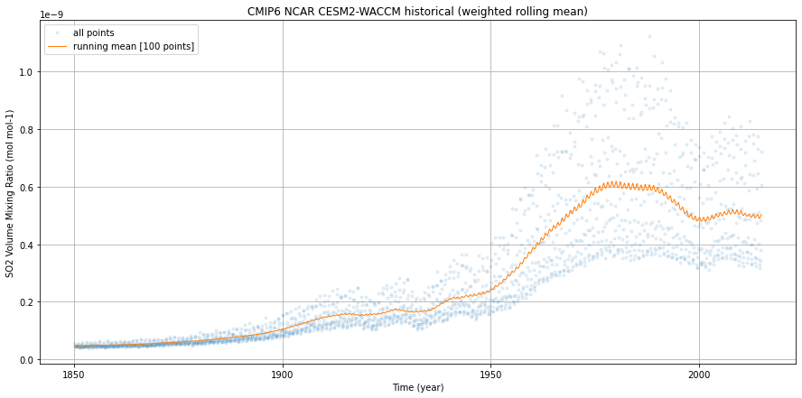
Visualize

%%time
fig = plt.figure(1, figsize=[15,7])

ax = plt.subplot(1, 1, 1)

weighted_mean.so2.plot(ax=ax,
             marker='.',
             linewidth=0,
             label = 'all points',
             alpha=.1
            )

dpmean.so2.plot(ax=ax,
             marker='',
             linewidth=1,
             label = 'running mean [100 points]'
            )
ax.legend()
ax.grid()
ax.set_ylabel(dset.so2.attrs['long_name'] + ' (' + dset.so2.attrs['units'] + ')')
ax.set_xlabel('Time (year)')
ax.set_title('CMIP6 NCAR CESM2-WACCM historical (weighted rolling mean)')
plt.savefig('CMIP_NCAR_CESM2-WACCM_historical_weighted_rolling_mean.png')

CPU times: user 570 ms, sys: 113 ms, total: 683 ms
Wall time: 682 ms

Save Results

To improve the reproducibility of our work (first for ourselves!), we need to keep track of all our work and ease its reuse. We will:

• Save this Jupyter notebook

• Save weighted mean

• Save rolling mean

• Save figure

We save intermediate results as netCDF files because they are small and ca be easily re-loaded (even if stored on cloud storage).

Save results locally

• Useful for further analysis but can be lost if you close your JupyterLab or if there is any problem with your JupyterLab instance

weighted_mean.to_netcdf('CMIP_NCAR_CESM2-WACCM_historical_weighted_mean.nc')

dpmean.to_netcdf('CMIP_NCAR_CESM2-WACCM_historical_rolling_mean.nc')

Save your results on NIRD (Norwegian infrastructure for Research Data)

• your credentials are in $HOME/.aws/credentials

• check with your instructor to get the secret access key (replace XXX by the right key)

[default]
aws_access_key_id=forces2021-work
aws_secret_access_key=XXXXXXXXXXXX
aws_endpoint_url=https://forces2021.uiogeo-apps.sigma2.no/

It is important to save yoru results in a place that can last longer than a few days/weeks!

import s3fs

fsg = s3fs.S3FileSystem(anon=False,
      client_kwargs={
         'endpoint_url': 'https://forces2021.uiogeo-apps.sigma2.no/'
      })

Set “remote” path (update annefou by your username) and save weighted mean as netCDF file

s3_path =  "s3://work/annefou/CMIP_NCAR_CESM2-WACCM_historical_weighted_mean.nc"
print(s3_path)

s3://work/annefou/CMIP_NCAR_CESM2-WACCM_historical_weighted_mean.nc

with fsg.open(s3_path, 'wb') as f:
    f.write(weighted_mean.to_netcdf(None))

Save rolling mean to remote location (update annefou with your username)

s3_path =  "s3://work/annefou/CMIP_NCAR_CESM2-WACCM_historical_rolling_mean.nc"
print(s3_path)

s3://work/annefou/CMIP_NCAR_CESM2-WACCM_historical_rolling_mean.nc

with fsg.open(s3_path, 'wb') as f:
    f.write(dpmean.to_netcdf(None))

Upload existing png file to remote s3 location

s3_path =  "s3://work/annefou/CMIP_NCAR_CESM2-WACCM_historical_weighted_rolling_mean.png"
print(s3_path)

s3://work/annefou/CMIP_NCAR_CESM2-WACCM_historical_weighted_rolling_mean.png

fsg.put('CMIP_NCAR_CESM2-WACCM_historical_weighted_rolling_mean.png', s3_path)

previous

Using xarray to read EBAS data

next

Using masks and computing weighted average