Some tips with xarray and pandas
Contents
Some tips with xarray and pandas
We have massively different levels here
Try to make some aims for technical skills you can learn!
If you are beginning with python –> learn the basics
If you are good at basic python –> learn new packages
If you know all the packages –> improve your skills with producing your own software etc.
If you don’t know git and github –> get better at this!
What are pandas and xarray?
Pandas –> like a spreadsheet 2D data with columns and rows
xarray –> like pandas, but in N dimensions
!wget 'https://zenodo.org/record/5639504/files/OsloAeroSec2011-3_subset2.nc'
--2021-11-02 19:12:35--  https://zenodo.org/record/5639504/files/OsloAeroSec2011-3_subset2.nc
Resolving zenodo.org (zenodo.org)... 137.138.76.77
Connecting to zenodo.org (zenodo.org)|137.138.76.77|:443... connected.
HTTP request sent, awaiting response... 200 OK
Length: 177021566 (169M) [application/octet-stream]
Saving to: ‘OsloAeroSec2011-3_subset2.nc’

OsloAeroSec2011-3_s 100%[===================>] 168.82M  12.9MB/s    in 6.3s

2021-11-02 19:12:42 (26.7 MB/s) - ‘OsloAeroSec2011-3_subset2.nc’ saved [177021566/177021566]
Some examples with xarray and pandas:
import xarray as xr
import numpy as np
import matplotlib.pyplot as plt
import pandas as pd
import datetime
import seaborn as sns
Reading in the data:
path='OsloAeroSec2011-3_subset2.nc'
ds = xr.open_dataset(path)
Opening multiple files:
list_of_files = [
    'file1.nc',
    'file2.nc'
]
xr.open_mfdataset(list_of_files, concat_dim='time',combine='by_coords')
Check how your dataset looks
Different types of information/data:
Coordinates
Data variables
Global attributes
Variable attributes
ds
<xarray.Dataset>
Dimensions:  (lat: 96, lev: 32, lon: 144, time: 36)
Coordinates:
  * lat      (lat) float64 -90.0 -88.11 -86.21 -84.32 ... 84.32 86.21 88.11 90.0
  * lon      (lon) float64 0.0 2.5 5.0 7.5 10.0 ... 350.0 352.5 355.0 357.5
  * lev      (lev) float64 3.643 7.595 14.36 24.61 ... 936.2 957.5 976.3 992.6
  * time     (time) datetime64[ns] 2011-02-01 2011-03-01 ... 2014-01-01
Data variables:
    hyam     (lev) float64 0.003643 0.007595 0.01436 ... 0.006255 0.001989 0.0
    hybm     (lev) float64 0.0 0.0 0.0 0.0 0.0 ... 0.9251 0.9512 0.9743 0.9926
    P0       float64 1e+05
    N_AER    (time, lev, lat, lon) float32 ...
    PS       (time, lat, lon) float32 ...
    T        (time, lev, lat, lon) float32 ...
    U        (time, lev, lat, lon) float32 ...
    V        (time, lev, lat, lon) float32 ...
Attributes:
    Conventions:       CF-1.0
    source:            CAM
    case:              OsloAeroSec_intBVOC_f19_f19
    logname:           x_sarbl
    host:
    initial_file:      OsloAero_intBVOC_f19_f19_spinup.cam.i.2011-01-01-00000.nc
    topography_file:   /proj/cesm_input-data/inputdata/noresm-only/inputForNu...
    model_doi_url:     https://doi.org/10.5065/D67H1H0V
    time_period_freq:  month_1
    history:           Tue Nov  2 08:04:41 2021: ncrcat -v T,N_AER,V,U atm/hi...
NCO: netCDF Operators version 4.7.9 (Homepage = http://nco....- lat: 96
- lev: 32
- lon: 144
- time: 36
- lat(lat)float64-90.0 -88.11 -86.21 ... 88.11 90.0
- long_name :
- latitude
- units :
- degrees_north
array([-90. , -88.105263, -86.210526, -84.315789, -82.421053, -80.526316, -78.631579, -76.736842, -74.842105, -72.947368, -71.052632, -69.157895, -67.263158, -65.368421, -63.473684, -61.578947, -59.684211, -57.789474, -55.894737, -54. , -52.105263, -50.210526, -48.315789, -46.421053, -44.526316, -42.631579, -40.736842, -38.842105, -36.947368, -35.052632, -33.157895, -31.263158, -29.368421, -27.473684, -25.578947, -23.684211, -21.789474, -19.894737, -18. , -16.105263, -14.210526, -12.315789, -10.421053, -8.526316, -6.631579, -4.736842, -2.842105, -0.947368, 0.947368, 2.842105, 4.736842, 6.631579, 8.526316, 10.421053, 12.315789, 14.210526, 16.105263, 18. , 19.894737, 21.789474, 23.684211, 25.578947, 27.473684, 29.368421, 31.263158, 33.157895, 35.052632, 36.947368, 38.842105, 40.736842, 42.631579, 44.526316, 46.421053, 48.315789, 50.210526, 52.105263, 54. , 55.894737, 57.789474, 59.684211, 61.578947, 63.473684, 65.368421, 67.263158, 69.157895, 71.052632, 72.947368, 74.842105, 76.736842, 78.631579, 80.526316, 82.421053, 84.315789, 86.210526, 88.105263, 90. ]) - lon(lon)float640.0 2.5 5.0 ... 352.5 355.0 357.5
- long_name :
- longitude
- units :
- degrees_east
array([ 0. , 2.5, 5. , 7.5, 10. , 12.5, 15. , 17.5, 20. , 22.5, 25. , 27.5, 30. , 32.5, 35. , 37.5, 40. , 42.5, 45. , 47.5, 50. , 52.5, 55. , 57.5, 60. , 62.5, 65. , 67.5, 70. , 72.5, 75. , 77.5, 80. , 82.5, 85. , 87.5, 90. , 92.5, 95. , 97.5, 100. , 102.5, 105. , 107.5, 110. , 112.5, 115. , 117.5, 120. , 122.5, 125. , 127.5, 130. , 132.5, 135. , 137.5, 140. , 142.5, 145. , 147.5, 150. , 152.5, 155. , 157.5, 160. , 162.5, 165. , 167.5, 170. , 172.5, 175. , 177.5, 180. , 182.5, 185. , 187.5, 190. , 192.5, 195. , 197.5, 200. , 202.5, 205. , 207.5, 210. , 212.5, 215. , 217.5, 220. , 222.5, 225. , 227.5, 230. , 232.5, 235. , 237.5, 240. , 242.5, 245. , 247.5, 250. , 252.5, 255. , 257.5, 260. , 262.5, 265. , 267.5, 270. , 272.5, 275. , 277.5, 280. , 282.5, 285. , 287.5, 290. , 292.5, 295. , 297.5, 300. , 302.5, 305. , 307.5, 310. , 312.5, 315. , 317.5, 320. , 322.5, 325. , 327.5, 330. , 332.5, 335. , 337.5, 340. , 342.5, 345. , 347.5, 350. , 352.5, 355. , 357.5]) - lev(lev)float643.643 7.595 14.36 ... 976.3 992.6
- long_name :
- hybrid level at midpoints (1000*(A+B))
- units :
- hPa
- positive :
- down
- standard_name :
- atmosphere_hybrid_sigma_pressure_coordinate
- formula_terms :
- a: hyam b: hybm p0: P0 ps: PS
array([ 3.643466, 7.59482 , 14.356632, 24.61222 , 35.92325 , 43.19375 , 51.677499, 61.520498, 73.750958, 87.82123 , 103.317127, 121.547241, 142.994039, 168.22508 , 197.908087, 232.828619, 273.910817, 322.241902, 379.100904, 445.992574, 524.687175, 609.778695, 691.38943 , 763.404481, 820.858369, 859.534767, 887.020249, 912.644547, 936.198398, 957.48548 , 976.325407, 992.556095]) - time(time)datetime64[ns]2011-02-01 ... 2014-01-01
- long_name :
- time
- bounds :
- time_bnds
array(['2011-02-01T00:00:00.000000000', '2011-03-01T00:00:00.000000000',
       '2011-04-01T00:00:00.000000000', '2011-05-01T00:00:00.000000000',
       '2011-06-01T00:00:00.000000000', '2011-07-01T00:00:00.000000000',
       '2011-08-01T00:00:00.000000000', '2011-09-01T00:00:00.000000000',
       '2011-10-01T00:00:00.000000000', '2011-11-01T00:00:00.000000000',
       '2011-12-01T00:00:00.000000000', '2012-01-01T00:00:00.000000000',
       '2012-02-01T00:00:00.000000000', '2012-03-01T00:00:00.000000000',
       '2012-04-01T00:00:00.000000000', '2012-05-01T00:00:00.000000000',
       '2012-06-01T00:00:00.000000000', '2012-07-01T00:00:00.000000000',
       '2012-08-01T00:00:00.000000000', '2012-09-01T00:00:00.000000000',
       '2012-10-01T00:00:00.000000000', '2012-11-01T00:00:00.000000000',
       '2012-12-01T00:00:00.000000000', '2013-01-01T00:00:00.000000000',
       '2013-02-01T00:00:00.000000000', '2013-03-01T00:00:00.000000000',
       '2013-04-01T00:00:00.000000000', '2013-05-01T00:00:00.000000000',
       '2013-06-01T00:00:00.000000000', '2013-07-01T00:00:00.000000000',
       '2013-08-01T00:00:00.000000000', '2013-09-01T00:00:00.000000000',
       '2013-10-01T00:00:00.000000000', '2013-11-01T00:00:00.000000000',
       '2013-12-01T00:00:00.000000000', '2014-01-01T00:00:00.000000000'],
      dtype='datetime64[ns]')
- hyam(lev)float64...
- long_name :
- hybrid A coefficient at layer midpoints
array([0.003643, 0.007595, 0.014357, 0.024612, 0.035923, 0.043194, 0.051677, 0.06152 , 0.073751, 0.087821, 0.103317, 0.121547, 0.142994, 0.168225, 0.178231, 0.170324, 0.161023, 0.15008 , 0.137207, 0.122062, 0.104245, 0.084979, 0.066502, 0.050197, 0.037189, 0.028432, 0.022209, 0.016407, 0.011075, 0.006255, 0.001989, 0. ]) - hybm(lev)float64...
- long_name :
- hybrid B coefficient at layer midpoints
array([0. , 0. , 0. , 0. , 0. , 0. , 0. , 0. , 0. , 0. , 0. , 0. , 0. , 0. , 0.019677, 0.062504, 0.112888, 0.172162, 0.241894, 0.323931, 0.420442, 0.5248 , 0.624888, 0.713208, 0.78367 , 0.831103, 0.864811, 0.896237, 0.925124, 0.951231, 0.974336, 0.992556]) - P0()float64...
- long_name :
- reference pressure
- units :
- Pa
array(100000.)
- N_AER(time, lev, lat, lon)float32...
- mdims :
- 1
- units :
- unitless
- long_name :
- Aerosol number concentration
- cell_methods :
- time: mean
[15925248 values with dtype=float32]
- PS(time, lat, lon)float32...
- units :
- Pa
- long_name :
- Surface pressure
- cell_methods :
- time: mean
[497664 values with dtype=float32]
- T(time, lev, lat, lon)float32...
- mdims :
- 1
- units :
- K
- long_name :
- Temperature
- cell_methods :
- time: mean
[15925248 values with dtype=float32]
- U(time, lev, lat, lon)float32...
- mdims :
- 1
- units :
- m/s
- long_name :
- Zonal wind
- cell_methods :
- time: mean
[15925248 values with dtype=float32]
- V(time, lev, lat, lon)float32...
- mdims :
- 1
- units :
- m/s
- long_name :
- Meridional wind
- cell_methods :
- time: mean
[15925248 values with dtype=float32]
- Conventions :
- CF-1.0
- source :
- CAM
- case :
- OsloAeroSec_intBVOC_f19_f19
- logname :
- x_sarbl
- host :
- initial_file :
- OsloAero_intBVOC_f19_f19_spinup.cam.i.2011-01-01-00000.nc
- topography_file :
- /proj/cesm_input-data/inputdata/noresm-only/inputForNudging/ERA_f19_tn14/ERA_bnd_topo.nc
- model_doi_url :
- https://doi.org/10.5065/D67H1H0V
- time_period_freq :
- month_1
- history :
- Tue Nov 2 08:04:41 2021: ncrcat -v T,N_AER,V,U atm/hist/OsloAeroSec_intBVOC_f19_f19.cam.h0.2011-01.nc atm/hist/OsloAeroSec_intBVOC_f19_f19.cam.h0.2011-02.nc atm/hist/OsloAeroSec_intBVOC_f19_f19.cam.h0.2011-03.nc atm/hist/OsloAeroSec_intBVOC_f19_f19.cam.h0.2011-04.nc atm/hist/OsloAeroSec_intBVOC_f19_f19.cam.h0.2011-05.nc atm/hist/OsloAeroSec_intBVOC_f19_f19.cam.h0.2011-06.nc atm/hist/OsloAeroSec_intBVOC_f19_f19.cam.h0.2011-07.nc atm/hist/OsloAeroSec_intBVOC_f19_f19.cam.h0.2011-08.nc atm/hist/OsloAeroSec_intBVOC_f19_f19.cam.h0.2011-09.nc atm/hist/OsloAeroSec_intBVOC_f19_f19.cam.h0.2011-10.nc atm/hist/OsloAeroSec_intBVOC_f19_f19.cam.h0.2011-11.nc atm/hist/OsloAeroSec_intBVOC_f19_f19.cam.h0.2011-12.nc atm/hist/OsloAeroSec_intBVOC_f19_f19.cam.h0.2012-01.nc atm/hist/OsloAeroSec_intBVOC_f19_f19.cam.h0.2012-02.nc atm/hist/OsloAeroSec_intBVOC_f19_f19.cam.h0.2012-03.nc atm/hist/OsloAeroSec_intBVOC_f19_f19.cam.h0.2012-04.nc atm/hist/OsloAeroSec_intBVOC_f19_f19.cam.h0.2012-05.nc atm/hist/OsloAeroSec_intBVOC_f19_f19.cam.h0.2012-06.nc atm/hist/OsloAeroSec_intBVOC_f19_f19.cam.h0.2012-07.nc atm/hist/OsloAeroSec_intBVOC_f19_f19.cam.h0.2012-08.nc atm/hist/OsloAeroSec_intBVOC_f19_f19.cam.h0.2012-09.nc atm/hist/OsloAeroSec_intBVOC_f19_f19.cam.h0.2012-10.nc atm/hist/OsloAeroSec_intBVOC_f19_f19.cam.h0.2012-11.nc atm/hist/OsloAeroSec_intBVOC_f19_f19.cam.h0.2012-12.nc atm/hist/OsloAeroSec_intBVOC_f19_f19.cam.h0.2013-01.nc atm/hist/OsloAeroSec_intBVOC_f19_f19.cam.h0.2013-02.nc atm/hist/OsloAeroSec_intBVOC_f19_f19.cam.h0.2013-03.nc atm/hist/OsloAeroSec_intBVOC_f19_f19.cam.h0.2013-04.nc atm/hist/OsloAeroSec_intBVOC_f19_f19.cam.h0.2013-05.nc atm/hist/OsloAeroSec_intBVOC_f19_f19.cam.h0.2013-06.nc atm/hist/OsloAeroSec_intBVOC_f19_f19.cam.h0.2013-07.nc atm/hist/OsloAeroSec_intBVOC_f19_f19.cam.h0.2013-08.nc atm/hist/OsloAeroSec_intBVOC_f19_f19.cam.h0.2013-09.nc atm/hist/OsloAeroSec_intBVOC_f19_f19.cam.h0.2013-10.nc atm/hist/OsloAeroSec_intBVOC_f19_f19.cam.h0.2013-11.nc atm/hist/OsloAeroSec_intBVOC_f19_f19.cam.h0.2013-12.nc OsloAeroSec2011-3_subset.nc
- NCO :
- netCDF Operators version 4.7.9 (Homepage = http://nco.sf.net, Code = http://github.com/nco/nco)
Sometimes we want to do some nice tweaks before we start:
ds['T']
<xarray.DataArray 'T' (time: 36, lev: 32, lat: 96, lon: 144)>
[15925248 values with dtype=float32]
Coordinates:
  * lat      (lat) float64 -90.0 -88.11 -86.21 -84.32 ... 84.32 86.21 88.11 90.0
  * lon      (lon) float64 0.0 2.5 5.0 7.5 10.0 ... 350.0 352.5 355.0 357.5
  * lev      (lev) float64 3.643 7.595 14.36 24.61 ... 936.2 957.5 976.3 992.6
  * time     (time) datetime64[ns] 2011-02-01 2011-03-01 ... 2014-01-01
Attributes:
    mdims:         1
    units:         K
    long_name:     Temperature
cell_methods: time: mean- time: 36
- lev: 32
- lat: 96
- lon: 144
- ...
[15925248 values with dtype=float32]
- lat(lat)float64-90.0 -88.11 -86.21 ... 88.11 90.0
- long_name :
- latitude
- units :
- degrees_north
array([-90. , -88.105263, -86.210526, -84.315789, -82.421053, -80.526316, -78.631579, -76.736842, -74.842105, -72.947368, -71.052632, -69.157895, -67.263158, -65.368421, -63.473684, -61.578947, -59.684211, -57.789474, -55.894737, -54. , -52.105263, -50.210526, -48.315789, -46.421053, -44.526316, -42.631579, -40.736842, -38.842105, -36.947368, -35.052632, -33.157895, -31.263158, -29.368421, -27.473684, -25.578947, -23.684211, -21.789474, -19.894737, -18. , -16.105263, -14.210526, -12.315789, -10.421053, -8.526316, -6.631579, -4.736842, -2.842105, -0.947368, 0.947368, 2.842105, 4.736842, 6.631579, 8.526316, 10.421053, 12.315789, 14.210526, 16.105263, 18. , 19.894737, 21.789474, 23.684211, 25.578947, 27.473684, 29.368421, 31.263158, 33.157895, 35.052632, 36.947368, 38.842105, 40.736842, 42.631579, 44.526316, 46.421053, 48.315789, 50.210526, 52.105263, 54. , 55.894737, 57.789474, 59.684211, 61.578947, 63.473684, 65.368421, 67.263158, 69.157895, 71.052632, 72.947368, 74.842105, 76.736842, 78.631579, 80.526316, 82.421053, 84.315789, 86.210526, 88.105263, 90. ]) - lon(lon)float640.0 2.5 5.0 ... 352.5 355.0 357.5
- long_name :
- longitude
- units :
- degrees_east
array([ 0. , 2.5, 5. , 7.5, 10. , 12.5, 15. , 17.5, 20. , 22.5, 25. , 27.5, 30. , 32.5, 35. , 37.5, 40. , 42.5, 45. , 47.5, 50. , 52.5, 55. , 57.5, 60. , 62.5, 65. , 67.5, 70. , 72.5, 75. , 77.5, 80. , 82.5, 85. , 87.5, 90. , 92.5, 95. , 97.5, 100. , 102.5, 105. , 107.5, 110. , 112.5, 115. , 117.5, 120. , 122.5, 125. , 127.5, 130. , 132.5, 135. , 137.5, 140. , 142.5, 145. , 147.5, 150. , 152.5, 155. , 157.5, 160. , 162.5, 165. , 167.5, 170. , 172.5, 175. , 177.5, 180. , 182.5, 185. , 187.5, 190. , 192.5, 195. , 197.5, 200. , 202.5, 205. , 207.5, 210. , 212.5, 215. , 217.5, 220. , 222.5, 225. , 227.5, 230. , 232.5, 235. , 237.5, 240. , 242.5, 245. , 247.5, 250. , 252.5, 255. , 257.5, 260. , 262.5, 265. , 267.5, 270. , 272.5, 275. , 277.5, 280. , 282.5, 285. , 287.5, 290. , 292.5, 295. , 297.5, 300. , 302.5, 305. , 307.5, 310. , 312.5, 315. , 317.5, 320. , 322.5, 325. , 327.5, 330. , 332.5, 335. , 337.5, 340. , 342.5, 345. , 347.5, 350. , 352.5, 355. , 357.5]) - lev(lev)float643.643 7.595 14.36 ... 976.3 992.6
- long_name :
- hybrid level at midpoints (1000*(A+B))
- units :
- hPa
- positive :
- down
- standard_name :
- atmosphere_hybrid_sigma_pressure_coordinate
- formula_terms :
- a: hyam b: hybm p0: P0 ps: PS
array([ 3.643466, 7.59482 , 14.356632, 24.61222 , 35.92325 , 43.19375 , 51.677499, 61.520498, 73.750958, 87.82123 , 103.317127, 121.547241, 142.994039, 168.22508 , 197.908087, 232.828619, 273.910817, 322.241902, 379.100904, 445.992574, 524.687175, 609.778695, 691.38943 , 763.404481, 820.858369, 859.534767, 887.020249, 912.644547, 936.198398, 957.48548 , 976.325407, 992.556095]) - time(time)datetime64[ns]2011-02-01 ... 2014-01-01
- long_name :
- time
- bounds :
- time_bnds
array(['2011-02-01T00:00:00.000000000', '2011-03-01T00:00:00.000000000',
       '2011-04-01T00:00:00.000000000', '2011-05-01T00:00:00.000000000',
       '2011-06-01T00:00:00.000000000', '2011-07-01T00:00:00.000000000',
       '2011-08-01T00:00:00.000000000', '2011-09-01T00:00:00.000000000',
       '2011-10-01T00:00:00.000000000', '2011-11-01T00:00:00.000000000',
       '2011-12-01T00:00:00.000000000', '2012-01-01T00:00:00.000000000',
       '2012-02-01T00:00:00.000000000', '2012-03-01T00:00:00.000000000',
       '2012-04-01T00:00:00.000000000', '2012-05-01T00:00:00.000000000',
       '2012-06-01T00:00:00.000000000', '2012-07-01T00:00:00.000000000',
       '2012-08-01T00:00:00.000000000', '2012-09-01T00:00:00.000000000',
       '2012-10-01T00:00:00.000000000', '2012-11-01T00:00:00.000000000',
       '2012-12-01T00:00:00.000000000', '2013-01-01T00:00:00.000000000',
       '2013-02-01T00:00:00.000000000', '2013-03-01T00:00:00.000000000',
       '2013-04-01T00:00:00.000000000', '2013-05-01T00:00:00.000000000',
       '2013-06-01T00:00:00.000000000', '2013-07-01T00:00:00.000000000',
       '2013-08-01T00:00:00.000000000', '2013-09-01T00:00:00.000000000',
       '2013-10-01T00:00:00.000000000', '2013-11-01T00:00:00.000000000',
       '2013-12-01T00:00:00.000000000', '2014-01-01T00:00:00.000000000'],
      dtype='datetime64[ns]')
- mdims :
- 1
- units :
- K
- long_name :
- Temperature
- cell_methods :
- time: mean
Assign attributes! Nice for plotting and to keep track of what is in your dataset (especially ‘units’ and ‘standard_name’/’long_name’ will be looked for by xarray.
ds['T_C'] = ds['T']-273.15

ds['T_C'] = ds['T_C'].assign_attrs({'units': '$^\circ$C'})
May always be small things you need to adjust:
ds['time']
<xarray.DataArray 'time' (time: 36)>
array(['2011-02-01T00:00:00.000000000', '2011-03-01T00:00:00.000000000',
       '2011-04-01T00:00:00.000000000', '2011-05-01T00:00:00.000000000',
       '2011-06-01T00:00:00.000000000', '2011-07-01T00:00:00.000000000',
       '2011-08-01T00:00:00.000000000', '2011-09-01T00:00:00.000000000',
       '2011-10-01T00:00:00.000000000', '2011-11-01T00:00:00.000000000',
       '2011-12-01T00:00:00.000000000', '2012-01-01T00:00:00.000000000',
       '2012-02-01T00:00:00.000000000', '2012-03-01T00:00:00.000000000',
       '2012-04-01T00:00:00.000000000', '2012-05-01T00:00:00.000000000',
       '2012-06-01T00:00:00.000000000', '2012-07-01T00:00:00.000000000',
       '2012-08-01T00:00:00.000000000', '2012-09-01T00:00:00.000000000',
       '2012-10-01T00:00:00.000000000', '2012-11-01T00:00:00.000000000',
       '2012-12-01T00:00:00.000000000', '2013-01-01T00:00:00.000000000',
       '2013-02-01T00:00:00.000000000', '2013-03-01T00:00:00.000000000',
       '2013-04-01T00:00:00.000000000', '2013-05-01T00:00:00.000000000',
       '2013-06-01T00:00:00.000000000', '2013-07-01T00:00:00.000000000',
       '2013-08-01T00:00:00.000000000', '2013-09-01T00:00:00.000000000',
       '2013-10-01T00:00:00.000000000', '2013-11-01T00:00:00.000000000',
       '2013-12-01T00:00:00.000000000', '2014-01-01T00:00:00.000000000'],
      dtype='datetime64[ns]')
Coordinates:
  * time     (time) datetime64[ns] 2011-02-01 2011-03-01 ... 2014-01-01
Attributes:
    long_name:  time
bounds: time_bnds- time: 36
- 2011-02-01 2011-03-01 2011-04-01 ... 2013-11-01 2013-12-01 2014-01-01
array(['2011-02-01T00:00:00.000000000', '2011-03-01T00:00:00.000000000', '2011-04-01T00:00:00.000000000', '2011-05-01T00:00:00.000000000', '2011-06-01T00:00:00.000000000', '2011-07-01T00:00:00.000000000', '2011-08-01T00:00:00.000000000', '2011-09-01T00:00:00.000000000', '2011-10-01T00:00:00.000000000', '2011-11-01T00:00:00.000000000', '2011-12-01T00:00:00.000000000', '2012-01-01T00:00:00.000000000', '2012-02-01T00:00:00.000000000', '2012-03-01T00:00:00.000000000', '2012-04-01T00:00:00.000000000', '2012-05-01T00:00:00.000000000', '2012-06-01T00:00:00.000000000', '2012-07-01T00:00:00.000000000', '2012-08-01T00:00:00.000000000', '2012-09-01T00:00:00.000000000', '2012-10-01T00:00:00.000000000', '2012-11-01T00:00:00.000000000', '2012-12-01T00:00:00.000000000', '2013-01-01T00:00:00.000000000', '2013-02-01T00:00:00.000000000', '2013-03-01T00:00:00.000000000', '2013-04-01T00:00:00.000000000', '2013-05-01T00:00:00.000000000', '2013-06-01T00:00:00.000000000', '2013-07-01T00:00:00.000000000', '2013-08-01T00:00:00.000000000', '2013-09-01T00:00:00.000000000', '2013-10-01T00:00:00.000000000', '2013-11-01T00:00:00.000000000', '2013-12-01T00:00:00.000000000', '2014-01-01T00:00:00.000000000'], dtype='datetime64[ns]') - time(time)datetime64[ns]2011-02-01 ... 2014-01-01
- long_name :
- time
- bounds :
- time_bnds
array(['2011-02-01T00:00:00.000000000', '2011-03-01T00:00:00.000000000',
       '2011-04-01T00:00:00.000000000', '2011-05-01T00:00:00.000000000',
       '2011-06-01T00:00:00.000000000', '2011-07-01T00:00:00.000000000',
       '2011-08-01T00:00:00.000000000', '2011-09-01T00:00:00.000000000',
       '2011-10-01T00:00:00.000000000', '2011-11-01T00:00:00.000000000',
       '2011-12-01T00:00:00.000000000', '2012-01-01T00:00:00.000000000',
       '2012-02-01T00:00:00.000000000', '2012-03-01T00:00:00.000000000',
       '2012-04-01T00:00:00.000000000', '2012-05-01T00:00:00.000000000',
       '2012-06-01T00:00:00.000000000', '2012-07-01T00:00:00.000000000',
       '2012-08-01T00:00:00.000000000', '2012-09-01T00:00:00.000000000',
       '2012-10-01T00:00:00.000000000', '2012-11-01T00:00:00.000000000',
       '2012-12-01T00:00:00.000000000', '2013-01-01T00:00:00.000000000',
       '2013-02-01T00:00:00.000000000', '2013-03-01T00:00:00.000000000',
       '2013-04-01T00:00:00.000000000', '2013-05-01T00:00:00.000000000',
       '2013-06-01T00:00:00.000000000', '2013-07-01T00:00:00.000000000',
       '2013-08-01T00:00:00.000000000', '2013-09-01T00:00:00.000000000',
       '2013-10-01T00:00:00.000000000', '2013-11-01T00:00:00.000000000',
       '2013-12-01T00:00:00.000000000', '2014-01-01T00:00:00.000000000'],
      dtype='datetime64[ns]')
- long_name :
- time
- bounds :
- time_bnds
This data in particular has an issue that the date is the end of the month, which gets read as the first of the next month. So I usually just to a quick fix and subtract roughly 15 days (half a month)
t_corrected= pd.to_datetime( ds['time'].values)- datetime.timedelta(days=15)
ds['time'] = t_corrected
ds['time']
<xarray.DataArray 'time' (time: 36)>
array(['2011-01-17T00:00:00.000000000', '2011-02-14T00:00:00.000000000',
       '2011-03-17T00:00:00.000000000', '2011-04-16T00:00:00.000000000',
       '2011-05-17T00:00:00.000000000', '2011-06-16T00:00:00.000000000',
       '2011-07-17T00:00:00.000000000', '2011-08-17T00:00:00.000000000',
       '2011-09-16T00:00:00.000000000', '2011-10-17T00:00:00.000000000',
       '2011-11-16T00:00:00.000000000', '2011-12-17T00:00:00.000000000',
       '2012-01-17T00:00:00.000000000', '2012-02-15T00:00:00.000000000',
       '2012-03-17T00:00:00.000000000', '2012-04-16T00:00:00.000000000',
       '2012-05-17T00:00:00.000000000', '2012-06-16T00:00:00.000000000',
       '2012-07-17T00:00:00.000000000', '2012-08-17T00:00:00.000000000',
       '2012-09-16T00:00:00.000000000', '2012-10-17T00:00:00.000000000',
       '2012-11-16T00:00:00.000000000', '2012-12-17T00:00:00.000000000',
       '2013-01-17T00:00:00.000000000', '2013-02-14T00:00:00.000000000',
       '2013-03-17T00:00:00.000000000', '2013-04-16T00:00:00.000000000',
       '2013-05-17T00:00:00.000000000', '2013-06-16T00:00:00.000000000',
       '2013-07-17T00:00:00.000000000', '2013-08-17T00:00:00.000000000',
       '2013-09-16T00:00:00.000000000', '2013-10-17T00:00:00.000000000',
       '2013-11-16T00:00:00.000000000', '2013-12-17T00:00:00.000000000'],
      dtype='datetime64[ns]')
Coordinates:
* time (time) datetime64[ns] 2011-01-17 2011-02-14 ... 2013-12-17- time: 36
- 2011-01-17 2011-02-14 2011-03-17 ... 2013-10-17 2013-11-16 2013-12-17
array(['2011-01-17T00:00:00.000000000', '2011-02-14T00:00:00.000000000', '2011-03-17T00:00:00.000000000', '2011-04-16T00:00:00.000000000', '2011-05-17T00:00:00.000000000', '2011-06-16T00:00:00.000000000', '2011-07-17T00:00:00.000000000', '2011-08-17T00:00:00.000000000', '2011-09-16T00:00:00.000000000', '2011-10-17T00:00:00.000000000', '2011-11-16T00:00:00.000000000', '2011-12-17T00:00:00.000000000', '2012-01-17T00:00:00.000000000', '2012-02-15T00:00:00.000000000', '2012-03-17T00:00:00.000000000', '2012-04-16T00:00:00.000000000', '2012-05-17T00:00:00.000000000', '2012-06-16T00:00:00.000000000', '2012-07-17T00:00:00.000000000', '2012-08-17T00:00:00.000000000', '2012-09-16T00:00:00.000000000', '2012-10-17T00:00:00.000000000', '2012-11-16T00:00:00.000000000', '2012-12-17T00:00:00.000000000', '2013-01-17T00:00:00.000000000', '2013-02-14T00:00:00.000000000', '2013-03-17T00:00:00.000000000', '2013-04-16T00:00:00.000000000', '2013-05-17T00:00:00.000000000', '2013-06-16T00:00:00.000000000', '2013-07-17T00:00:00.000000000', '2013-08-17T00:00:00.000000000', '2013-09-16T00:00:00.000000000', '2013-10-17T00:00:00.000000000', '2013-11-16T00:00:00.000000000', '2013-12-17T00:00:00.000000000'], dtype='datetime64[ns]') - time(time)datetime64[ns]2011-01-17 ... 2013-12-17
array(['2011-01-17T00:00:00.000000000', '2011-02-14T00:00:00.000000000',
       '2011-03-17T00:00:00.000000000', '2011-04-16T00:00:00.000000000',
       '2011-05-17T00:00:00.000000000', '2011-06-16T00:00:00.000000000',
       '2011-07-17T00:00:00.000000000', '2011-08-17T00:00:00.000000000',
       '2011-09-16T00:00:00.000000000', '2011-10-17T00:00:00.000000000',
       '2011-11-16T00:00:00.000000000', '2011-12-17T00:00:00.000000000',
       '2012-01-17T00:00:00.000000000', '2012-02-15T00:00:00.000000000',
       '2012-03-17T00:00:00.000000000', '2012-04-16T00:00:00.000000000',
       '2012-05-17T00:00:00.000000000', '2012-06-16T00:00:00.000000000',
       '2012-07-17T00:00:00.000000000', '2012-08-17T00:00:00.000000000',
       '2012-09-16T00:00:00.000000000', '2012-10-17T00:00:00.000000000',
       '2012-11-16T00:00:00.000000000', '2012-12-17T00:00:00.000000000',
       '2013-01-17T00:00:00.000000000', '2013-02-14T00:00:00.000000000',
       '2013-03-17T00:00:00.000000000', '2013-04-16T00:00:00.000000000',
       '2013-05-17T00:00:00.000000000', '2013-06-16T00:00:00.000000000',
       '2013-07-17T00:00:00.000000000', '2013-08-17T00:00:00.000000000',
       '2013-09-16T00:00:00.000000000', '2013-10-17T00:00:00.000000000',
       '2013-11-16T00:00:00.000000000', '2013-12-17T00:00:00.000000000'],
      dtype='datetime64[ns]')
Convert longitude:
this data comes in 0–360 degrees, but often -180 to 180 is more convenient. So we can convert:
NOTE: Maybe you want to put this in a module? Or a package..
ds
<xarray.Dataset>
Dimensions:  (lat: 96, lev: 32, lon: 144, time: 36)
Coordinates:
  * lat      (lat) float64 -90.0 -88.11 -86.21 -84.32 ... 84.32 86.21 88.11 90.0
  * lon      (lon) float64 0.0 2.5 5.0 7.5 10.0 ... 350.0 352.5 355.0 357.5
  * lev      (lev) float64 3.643 7.595 14.36 24.61 ... 936.2 957.5 976.3 992.6
  * time     (time) datetime64[ns] 2011-01-17 2011-02-14 ... 2013-12-17
Data variables:
    hyam     (lev) float64 0.003643 0.007595 0.01436 ... 0.006255 0.001989 0.0
    hybm     (lev) float64 0.0 0.0 0.0 0.0 0.0 ... 0.9251 0.9512 0.9743 0.9926
    P0       float64 1e+05
    N_AER    (time, lev, lat, lon) float32 ...
    PS       (time, lat, lon) float32 ...
    T        (time, lev, lat, lon) float32 268.3 268.3 268.3 ... 250.4 250.4
    U        (time, lev, lat, lon) float32 ...
    V        (time, lev, lat, lon) float32 ...
    T_C      (time, lev, lat, lon) float32 -4.89 -4.89 -4.89 ... -22.78 -22.78
Attributes:
    Conventions:       CF-1.0
    source:            CAM
    case:              OsloAeroSec_intBVOC_f19_f19
    logname:           x_sarbl
    host:
    initial_file:      OsloAero_intBVOC_f19_f19_spinup.cam.i.2011-01-01-00000.nc
    topography_file:   /proj/cesm_input-data/inputdata/noresm-only/inputForNu...
    model_doi_url:     https://doi.org/10.5065/D67H1H0V
    time_period_freq:  month_1
    history:           Tue Nov  2 08:04:41 2021: ncrcat -v T,N_AER,V,U atm/hi...
NCO: netCDF Operators version 4.7.9 (Homepage = http://nco....- lat: 96
- lev: 32
- lon: 144
- time: 36
- lat(lat)float64-90.0 -88.11 -86.21 ... 88.11 90.0
- long_name :
- latitude
- units :
- degrees_north
array([-90. , -88.105263, -86.210526, -84.315789, -82.421053, -80.526316, -78.631579, -76.736842, -74.842105, -72.947368, -71.052632, -69.157895, -67.263158, -65.368421, -63.473684, -61.578947, -59.684211, -57.789474, -55.894737, -54. , -52.105263, -50.210526, -48.315789, -46.421053, -44.526316, -42.631579, -40.736842, -38.842105, -36.947368, -35.052632, -33.157895, -31.263158, -29.368421, -27.473684, -25.578947, -23.684211, -21.789474, -19.894737, -18. , -16.105263, -14.210526, -12.315789, -10.421053, -8.526316, -6.631579, -4.736842, -2.842105, -0.947368, 0.947368, 2.842105, 4.736842, 6.631579, 8.526316, 10.421053, 12.315789, 14.210526, 16.105263, 18. , 19.894737, 21.789474, 23.684211, 25.578947, 27.473684, 29.368421, 31.263158, 33.157895, 35.052632, 36.947368, 38.842105, 40.736842, 42.631579, 44.526316, 46.421053, 48.315789, 50.210526, 52.105263, 54. , 55.894737, 57.789474, 59.684211, 61.578947, 63.473684, 65.368421, 67.263158, 69.157895, 71.052632, 72.947368, 74.842105, 76.736842, 78.631579, 80.526316, 82.421053, 84.315789, 86.210526, 88.105263, 90. ]) - lon(lon)float640.0 2.5 5.0 ... 352.5 355.0 357.5
- long_name :
- longitude
- units :
- degrees_east
array([ 0. , 2.5, 5. , 7.5, 10. , 12.5, 15. , 17.5, 20. , 22.5, 25. , 27.5, 30. , 32.5, 35. , 37.5, 40. , 42.5, 45. , 47.5, 50. , 52.5, 55. , 57.5, 60. , 62.5, 65. , 67.5, 70. , 72.5, 75. , 77.5, 80. , 82.5, 85. , 87.5, 90. , 92.5, 95. , 97.5, 100. , 102.5, 105. , 107.5, 110. , 112.5, 115. , 117.5, 120. , 122.5, 125. , 127.5, 130. , 132.5, 135. , 137.5, 140. , 142.5, 145. , 147.5, 150. , 152.5, 155. , 157.5, 160. , 162.5, 165. , 167.5, 170. , 172.5, 175. , 177.5, 180. , 182.5, 185. , 187.5, 190. , 192.5, 195. , 197.5, 200. , 202.5, 205. , 207.5, 210. , 212.5, 215. , 217.5, 220. , 222.5, 225. , 227.5, 230. , 232.5, 235. , 237.5, 240. , 242.5, 245. , 247.5, 250. , 252.5, 255. , 257.5, 260. , 262.5, 265. , 267.5, 270. , 272.5, 275. , 277.5, 280. , 282.5, 285. , 287.5, 290. , 292.5, 295. , 297.5, 300. , 302.5, 305. , 307.5, 310. , 312.5, 315. , 317.5, 320. , 322.5, 325. , 327.5, 330. , 332.5, 335. , 337.5, 340. , 342.5, 345. , 347.5, 350. , 352.5, 355. , 357.5]) - lev(lev)float643.643 7.595 14.36 ... 976.3 992.6
- long_name :
- hybrid level at midpoints (1000*(A+B))
- units :
- hPa
- positive :
- down
- standard_name :
- atmosphere_hybrid_sigma_pressure_coordinate
- formula_terms :
- a: hyam b: hybm p0: P0 ps: PS
array([ 3.643466, 7.59482 , 14.356632, 24.61222 , 35.92325 , 43.19375 , 51.677499, 61.520498, 73.750958, 87.82123 , 103.317127, 121.547241, 142.994039, 168.22508 , 197.908087, 232.828619, 273.910817, 322.241902, 379.100904, 445.992574, 524.687175, 609.778695, 691.38943 , 763.404481, 820.858369, 859.534767, 887.020249, 912.644547, 936.198398, 957.48548 , 976.325407, 992.556095]) - time(time)datetime64[ns]2011-01-17 ... 2013-12-17
array(['2011-01-17T00:00:00.000000000', '2011-02-14T00:00:00.000000000',
       '2011-03-17T00:00:00.000000000', '2011-04-16T00:00:00.000000000',
       '2011-05-17T00:00:00.000000000', '2011-06-16T00:00:00.000000000',
       '2011-07-17T00:00:00.000000000', '2011-08-17T00:00:00.000000000',
       '2011-09-16T00:00:00.000000000', '2011-10-17T00:00:00.000000000',
       '2011-11-16T00:00:00.000000000', '2011-12-17T00:00:00.000000000',
       '2012-01-17T00:00:00.000000000', '2012-02-15T00:00:00.000000000',
       '2012-03-17T00:00:00.000000000', '2012-04-16T00:00:00.000000000',
       '2012-05-17T00:00:00.000000000', '2012-06-16T00:00:00.000000000',
       '2012-07-17T00:00:00.000000000', '2012-08-17T00:00:00.000000000',
       '2012-09-16T00:00:00.000000000', '2012-10-17T00:00:00.000000000',
       '2012-11-16T00:00:00.000000000', '2012-12-17T00:00:00.000000000',
       '2013-01-17T00:00:00.000000000', '2013-02-14T00:00:00.000000000',
       '2013-03-17T00:00:00.000000000', '2013-04-16T00:00:00.000000000',
       '2013-05-17T00:00:00.000000000', '2013-06-16T00:00:00.000000000',
       '2013-07-17T00:00:00.000000000', '2013-08-17T00:00:00.000000000',
       '2013-09-16T00:00:00.000000000', '2013-10-17T00:00:00.000000000',
       '2013-11-16T00:00:00.000000000', '2013-12-17T00:00:00.000000000'],
      dtype='datetime64[ns]')
- hyam(lev)float640.003643 0.007595 ... 0.001989 0.0
- long_name :
- hybrid A coefficient at layer midpoints
array([0.003643, 0.007595, 0.014357, 0.024612, 0.035923, 0.043194, 0.051677, 0.06152 , 0.073751, 0.087821, 0.103317, 0.121547, 0.142994, 0.168225, 0.178231, 0.170324, 0.161023, 0.15008 , 0.137207, 0.122062, 0.104245, 0.084979, 0.066502, 0.050197, 0.037189, 0.028432, 0.022209, 0.016407, 0.011075, 0.006255, 0.001989, 0. ]) - hybm(lev)float640.0 0.0 0.0 ... 0.9743 0.9926
- long_name :
- hybrid B coefficient at layer midpoints
array([0. , 0. , 0. , 0. , 0. , 0. , 0. , 0. , 0. , 0. , 0. , 0. , 0. , 0. , 0.019677, 0.062504, 0.112888, 0.172162, 0.241894, 0.323931, 0.420442, 0.5248 , 0.624888, 0.713208, 0.78367 , 0.831103, 0.864811, 0.896237, 0.925124, 0.951231, 0.974336, 0.992556]) - P0()float641e+05
- long_name :
- reference pressure
- units :
- Pa
array(100000.)
- N_AER(time, lev, lat, lon)float32...
- mdims :
- 1
- units :
- unitless
- long_name :
- Aerosol number concentration
- cell_methods :
- time: mean
[15925248 values with dtype=float32]
- PS(time, lat, lon)float32...
- units :
- Pa
- long_name :
- Surface pressure
- cell_methods :
- time: mean
[497664 values with dtype=float32]
- T(time, lev, lat, lon)float32268.3 268.3 268.3 ... 250.4 250.4
- mdims :
- 1
- units :
- K
- long_name :
- Temperature
- cell_methods :
- time: mean
array([[[[268.25964, ..., 268.25964], ..., [221.06685, ..., 221.06685]], ..., [[249.0903 , ..., 249.08987], ..., [242.41449, ..., 242.41441]]], ..., [[[268.05267, ..., 268.05267], ..., [205.59595, ..., 205.59595]], ..., [[247.56898, ..., 247.56854], ..., [250.36978, ..., 250.36974]]]], dtype=float32) - U(time, lev, lat, lon)float32...
- mdims :
- 1
- units :
- m/s
- long_name :
- Zonal wind
- cell_methods :
- time: mean
[15925248 values with dtype=float32]
- V(time, lev, lat, lon)float32...
- mdims :
- 1
- units :
- m/s
- long_name :
- Meridional wind
- cell_methods :
- time: mean
[15925248 values with dtype=float32]
- T_C(time, lev, lat, lon)float32-4.89 -4.89 -4.89 ... -22.78 -22.78
- units :
- $^\circ$C
array([[[[ -4.8903503,  -4.8903503,  -4.8903503, ...,  -4.8903503,
           -4.8903503,  -4.8903503],
         [ -4.8196716,  -4.8223267,  -4.825165 , ...,  -4.8126526,
           -4.81485  ,  -4.817169 ],
         [ -4.83197  ,  -4.8335876,  -4.835602 , ...,  -4.8289795,
           -4.829651 ,  -4.830658 ],
         ...,
         [-55.792343 , -55.79561  , -55.795456 , ..., -55.761215 ,
          -55.77481  , -55.78546  ],
         [-54.191193 , -54.19098  , -54.189697 , ..., -54.18521  ,
          -54.188477 , -54.189896 ],
         [-52.083145 , -52.083145 , -52.083145 , ..., -52.083145 ,
          -52.083145 , -52.083145 ]],

        [[-23.739273 , -23.739273 , -23.739273 , ..., -23.739273 ,
          -23.739273 , -23.739273 ],
         [-23.767685 , -23.771576 , -23.775482 , ..., -23.75615  ,
          -23.759964 , -23.76381  ],
         [-23.807007 , -23.814346 , -23.821655 , ..., -23.784378 ,
          -23.792023 , -23.799591 ],
...
         [-20.15744  , -20.10225  , -20.037933 , ..., -20.343307 ,
          -20.293549 , -20.226944 ],
         [-20.300293 , -20.294968 , -20.28984  , ..., -20.338242 ,
          -20.327667 , -20.314743 ],
         [-21.674057 , -21.674057 , -21.674057 , ..., -21.674103 ,
          -21.674072 , -21.674072 ]],

        [[-25.581009 , -25.578247 , -25.577698 , ..., -25.581787 ,
          -25.581665 , -25.581451 ],
         [-24.850723 , -24.980194 , -25.107773 , ..., -24.482056 ,
          -24.600998 , -24.726486 ],
         [-24.219345 , -24.422455 , -24.651505 , ..., -23.474213 ,
          -23.701065 , -23.969467 ],
         ...,
         [-21.141861 , -20.991745 , -20.857666 , ..., -21.395355 ,
          -21.36232  , -21.275116 ],
         [-21.322876 , -21.310684 , -21.29712  , ..., -21.403366 ,
          -21.374374 , -21.343674 ],
         [-22.780212 , -22.780243 , -22.78032  , ..., -22.779892 ,
          -22.780273 , -22.780258 ]]]], dtype=float32)
- Conventions :
- CF-1.0
- source :
- CAM
- case :
- OsloAeroSec_intBVOC_f19_f19
- logname :
- x_sarbl
- host :
- initial_file :
- OsloAero_intBVOC_f19_f19_spinup.cam.i.2011-01-01-00000.nc
- topography_file :
- /proj/cesm_input-data/inputdata/noresm-only/inputForNudging/ERA_f19_tn14/ERA_bnd_topo.nc
- model_doi_url :
- https://doi.org/10.5065/D67H1H0V
- time_period_freq :
- month_1
- history :
- Tue Nov 2 08:04:41 2021: ncrcat -v T,N_AER,V,U atm/hist/OsloAeroSec_intBVOC_f19_f19.cam.h0.2011-01.nc atm/hist/OsloAeroSec_intBVOC_f19_f19.cam.h0.2011-02.nc atm/hist/OsloAeroSec_intBVOC_f19_f19.cam.h0.2011-03.nc atm/hist/OsloAeroSec_intBVOC_f19_f19.cam.h0.2011-04.nc atm/hist/OsloAeroSec_intBVOC_f19_f19.cam.h0.2011-05.nc atm/hist/OsloAeroSec_intBVOC_f19_f19.cam.h0.2011-06.nc atm/hist/OsloAeroSec_intBVOC_f19_f19.cam.h0.2011-07.nc atm/hist/OsloAeroSec_intBVOC_f19_f19.cam.h0.2011-08.nc atm/hist/OsloAeroSec_intBVOC_f19_f19.cam.h0.2011-09.nc atm/hist/OsloAeroSec_intBVOC_f19_f19.cam.h0.2011-10.nc atm/hist/OsloAeroSec_intBVOC_f19_f19.cam.h0.2011-11.nc atm/hist/OsloAeroSec_intBVOC_f19_f19.cam.h0.2011-12.nc atm/hist/OsloAeroSec_intBVOC_f19_f19.cam.h0.2012-01.nc atm/hist/OsloAeroSec_intBVOC_f19_f19.cam.h0.2012-02.nc atm/hist/OsloAeroSec_intBVOC_f19_f19.cam.h0.2012-03.nc atm/hist/OsloAeroSec_intBVOC_f19_f19.cam.h0.2012-04.nc atm/hist/OsloAeroSec_intBVOC_f19_f19.cam.h0.2012-05.nc atm/hist/OsloAeroSec_intBVOC_f19_f19.cam.h0.2012-06.nc atm/hist/OsloAeroSec_intBVOC_f19_f19.cam.h0.2012-07.nc atm/hist/OsloAeroSec_intBVOC_f19_f19.cam.h0.2012-08.nc atm/hist/OsloAeroSec_intBVOC_f19_f19.cam.h0.2012-09.nc atm/hist/OsloAeroSec_intBVOC_f19_f19.cam.h0.2012-10.nc atm/hist/OsloAeroSec_intBVOC_f19_f19.cam.h0.2012-11.nc atm/hist/OsloAeroSec_intBVOC_f19_f19.cam.h0.2012-12.nc atm/hist/OsloAeroSec_intBVOC_f19_f19.cam.h0.2013-01.nc atm/hist/OsloAeroSec_intBVOC_f19_f19.cam.h0.2013-02.nc atm/hist/OsloAeroSec_intBVOC_f19_f19.cam.h0.2013-03.nc atm/hist/OsloAeroSec_intBVOC_f19_f19.cam.h0.2013-04.nc atm/hist/OsloAeroSec_intBVOC_f19_f19.cam.h0.2013-05.nc atm/hist/OsloAeroSec_intBVOC_f19_f19.cam.h0.2013-06.nc atm/hist/OsloAeroSec_intBVOC_f19_f19.cam.h0.2013-07.nc atm/hist/OsloAeroSec_intBVOC_f19_f19.cam.h0.2013-08.nc atm/hist/OsloAeroSec_intBVOC_f19_f19.cam.h0.2013-09.nc atm/hist/OsloAeroSec_intBVOC_f19_f19.cam.h0.2013-10.nc atm/hist/OsloAeroSec_intBVOC_f19_f19.cam.h0.2013-11.nc atm/hist/OsloAeroSec_intBVOC_f19_f19.cam.h0.2013-12.nc OsloAeroSec2011-3_subset.nc
- NCO :
- netCDF Operators version 4.7.9 (Homepage = http://nco.sf.net, Code = http://github.com/nco/nco)
def convert360_180(_ds):
    """
    convert longitude from 0-360 to -180 -- 180 deg
    """
    # check if already
    attrs = _ds['lon'].attrs
    if _ds['lon'].min() >= 0:
        with xr.set_options(keep_attrs=True):
            _ds.coords['lon'] = (_ds['lon'] + 180) % 360 - 180
        _ds = _ds.sortby('lon')
    return _ds
(migth want to move this to a module!)
ds = convert360_180(ds)
ds['lon']
<xarray.DataArray 'lon' (lon: 144)>
array([-180. , -177.5, -175. , -172.5, -170. , -167.5, -165. , -162.5, -160. ,
       -157.5, -155. , -152.5, -150. , -147.5, -145. , -142.5, -140. , -137.5,
       -135. , -132.5, -130. , -127.5, -125. , -122.5, -120. , -117.5, -115. ,
       -112.5, -110. , -107.5, -105. , -102.5, -100. ,  -97.5,  -95. ,  -92.5,
        -90. ,  -87.5,  -85. ,  -82.5,  -80. ,  -77.5,  -75. ,  -72.5,  -70. ,
        -67.5,  -65. ,  -62.5,  -60. ,  -57.5,  -55. ,  -52.5,  -50. ,  -47.5,
        -45. ,  -42.5,  -40. ,  -37.5,  -35. ,  -32.5,  -30. ,  -27.5,  -25. ,
        -22.5,  -20. ,  -17.5,  -15. ,  -12.5,  -10. ,   -7.5,   -5. ,   -2.5,
          0. ,    2.5,    5. ,    7.5,   10. ,   12.5,   15. ,   17.5,   20. ,
         22.5,   25. ,   27.5,   30. ,   32.5,   35. ,   37.5,   40. ,   42.5,
         45. ,   47.5,   50. ,   52.5,   55. ,   57.5,   60. ,   62.5,   65. ,
         67.5,   70. ,   72.5,   75. ,   77.5,   80. ,   82.5,   85. ,   87.5,
         90. ,   92.5,   95. ,   97.5,  100. ,  102.5,  105. ,  107.5,  110. ,
        112.5,  115. ,  117.5,  120. ,  122.5,  125. ,  127.5,  130. ,  132.5,
        135. ,  137.5,  140. ,  142.5,  145. ,  147.5,  150. ,  152.5,  155. ,
        157.5,  160. ,  162.5,  165. ,  167.5,  170. ,  172.5,  175. ,  177.5])
Coordinates:
  * lon      (lon) float64 -180.0 -177.5 -175.0 -172.5 ... 172.5 175.0 177.5
Attributes:
    long_name:  longitude
units: degrees_east- lon: 144
- -180.0 -177.5 -175.0 -172.5 -170.0 ... 167.5 170.0 172.5 175.0 177.5
array([-180. , -177.5, -175. , -172.5, -170. , -167.5, -165. , -162.5, -160. , -157.5, -155. , -152.5, -150. , -147.5, -145. , -142.5, -140. , -137.5, -135. , -132.5, -130. , -127.5, -125. , -122.5, -120. , -117.5, -115. , -112.5, -110. , -107.5, -105. , -102.5, -100. , -97.5, -95. , -92.5, -90. , -87.5, -85. , -82.5, -80. , -77.5, -75. , -72.5, -70. , -67.5, -65. , -62.5, -60. , -57.5, -55. , -52.5, -50. , -47.5, -45. , -42.5, -40. , -37.5, -35. , -32.5, -30. , -27.5, -25. , -22.5, -20. , -17.5, -15. , -12.5, -10. , -7.5, -5. , -2.5, 0. , 2.5, 5. , 7.5, 10. , 12.5, 15. , 17.5, 20. , 22.5, 25. , 27.5, 30. , 32.5, 35. , 37.5, 40. , 42.5, 45. , 47.5, 50. , 52.5, 55. , 57.5, 60. , 62.5, 65. , 67.5, 70. , 72.5, 75. , 77.5, 80. , 82.5, 85. , 87.5, 90. , 92.5, 95. , 97.5, 100. , 102.5, 105. , 107.5, 110. , 112.5, 115. , 117.5, 120. , 122.5, 125. , 127.5, 130. , 132.5, 135. , 137.5, 140. , 142.5, 145. , 147.5, 150. , 152.5, 155. , 157.5, 160. , 162.5, 165. , 167.5, 170. , 172.5, 175. , 177.5]) - lon(lon)float64-180.0 -177.5 ... 175.0 177.5
- long_name :
- longitude
- units :
- degrees_east
array([-180. , -177.5, -175. , -172.5, -170. , -167.5, -165. , -162.5, -160. ,
       -157.5, -155. , -152.5, -150. , -147.5, -145. , -142.5, -140. , -137.5,
       -135. , -132.5, -130. , -127.5, -125. , -122.5, -120. , -117.5, -115. ,
       -112.5, -110. , -107.5, -105. , -102.5, -100. ,  -97.5,  -95. ,  -92.5,
        -90. ,  -87.5,  -85. ,  -82.5,  -80. ,  -77.5,  -75. ,  -72.5,  -70. ,
        -67.5,  -65. ,  -62.5,  -60. ,  -57.5,  -55. ,  -52.5,  -50. ,  -47.5,
        -45. ,  -42.5,  -40. ,  -37.5,  -35. ,  -32.5,  -30. ,  -27.5,  -25. ,
        -22.5,  -20. ,  -17.5,  -15. ,  -12.5,  -10. ,   -7.5,   -5. ,   -2.5,
          0. ,    2.5,    5. ,    7.5,   10. ,   12.5,   15. ,   17.5,   20. ,
         22.5,   25. ,   27.5,   30. ,   32.5,   35. ,   37.5,   40. ,   42.5,
         45. ,   47.5,   50. ,   52.5,   55. ,   57.5,   60. ,   62.5,   65. ,
         67.5,   70. ,   72.5,   75. ,   77.5,   80. ,   82.5,   85. ,   87.5,
         90. ,   92.5,   95. ,   97.5,  100. ,  102.5,  105. ,  107.5,  110. ,
        112.5,  115. ,  117.5,  120. ,  122.5,  125. ,  127.5,  130. ,  132.5,
        135. ,  137.5,  140. ,  142.5,  145. ,  147.5,  150. ,  152.5,  155. ,
        157.5,  160. ,  162.5,  165. ,  167.5,  170. ,  172.5,  175. ,  177.5])
- long_name :
- longitude
- units :
- degrees_east
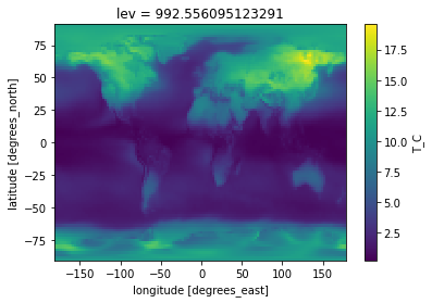
Let’s pick out only the surface layer. It’s the last one:
Selecting data and super quick plotting:
xarray loads data only when it needs to (it’s lazy, Anne can explain), and you might want to early on define the subset of data you want to look at so that you don’t end up loading a lot of extra data.
isel, sel
ds_s = ds.isel(lev=-1)
ds_s
<xarray.Dataset>
Dimensions:  (lat: 96, lon: 144, time: 36)
Coordinates:
  * lat      (lat) float64 -90.0 -88.11 -86.21 -84.32 ... 84.32 86.21 88.11 90.0
  * lon      (lon) float64 -180.0 -177.5 -175.0 -172.5 ... 172.5 175.0 177.5
    lev      float64 992.6
  * time     (time) datetime64[ns] 2011-01-17 2011-02-14 ... 2013-12-17
Data variables:
    hyam     float64 0.0
    hybm     float64 0.9926
    P0       float64 1e+05
    N_AER    (time, lat, lon) float32 ...
    PS       (time, lat, lon) float32 ...
    T        (time, lat, lon) float32 249.1 249.1 249.1 ... 250.4 250.4 250.4
    U        (time, lat, lon) float32 ...
    V        (time, lat, lon) float32 ...
    T_C      (time, lat, lon) float32 -24.04 -24.04 -24.04 ... -22.78 -22.78
Attributes:
    Conventions:       CF-1.0
    source:            CAM
    case:              OsloAeroSec_intBVOC_f19_f19
    logname:           x_sarbl
    host:
    initial_file:      OsloAero_intBVOC_f19_f19_spinup.cam.i.2011-01-01-00000.nc
    topography_file:   /proj/cesm_input-data/inputdata/noresm-only/inputForNu...
    model_doi_url:     https://doi.org/10.5065/D67H1H0V
    time_period_freq:  month_1
    history:           Tue Nov  2 08:04:41 2021: ncrcat -v T,N_AER,V,U atm/hi...
NCO: netCDF Operators version 4.7.9 (Homepage = http://nco....- lat: 96
- lon: 144
- time: 36
- lat(lat)float64-90.0 -88.11 -86.21 ... 88.11 90.0
- long_name :
- latitude
- units :
- degrees_north
array([-90. , -88.105263, -86.210526, -84.315789, -82.421053, -80.526316, -78.631579, -76.736842, -74.842105, -72.947368, -71.052632, -69.157895, -67.263158, -65.368421, -63.473684, -61.578947, -59.684211, -57.789474, -55.894737, -54. , -52.105263, -50.210526, -48.315789, -46.421053, -44.526316, -42.631579, -40.736842, -38.842105, -36.947368, -35.052632, -33.157895, -31.263158, -29.368421, -27.473684, -25.578947, -23.684211, -21.789474, -19.894737, -18. , -16.105263, -14.210526, -12.315789, -10.421053, -8.526316, -6.631579, -4.736842, -2.842105, -0.947368, 0.947368, 2.842105, 4.736842, 6.631579, 8.526316, 10.421053, 12.315789, 14.210526, 16.105263, 18. , 19.894737, 21.789474, 23.684211, 25.578947, 27.473684, 29.368421, 31.263158, 33.157895, 35.052632, 36.947368, 38.842105, 40.736842, 42.631579, 44.526316, 46.421053, 48.315789, 50.210526, 52.105263, 54. , 55.894737, 57.789474, 59.684211, 61.578947, 63.473684, 65.368421, 67.263158, 69.157895, 71.052632, 72.947368, 74.842105, 76.736842, 78.631579, 80.526316, 82.421053, 84.315789, 86.210526, 88.105263, 90. ]) - lon(lon)float64-180.0 -177.5 ... 175.0 177.5
- long_name :
- longitude
- units :
- degrees_east
array([-180. , -177.5, -175. , -172.5, -170. , -167.5, -165. , -162.5, -160. , -157.5, -155. , -152.5, -150. , -147.5, -145. , -142.5, -140. , -137.5, -135. , -132.5, -130. , -127.5, -125. , -122.5, -120. , -117.5, -115. , -112.5, -110. , -107.5, -105. , -102.5, -100. , -97.5, -95. , -92.5, -90. , -87.5, -85. , -82.5, -80. , -77.5, -75. , -72.5, -70. , -67.5, -65. , -62.5, -60. , -57.5, -55. , -52.5, -50. , -47.5, -45. , -42.5, -40. , -37.5, -35. , -32.5, -30. , -27.5, -25. , -22.5, -20. , -17.5, -15. , -12.5, -10. , -7.5, -5. , -2.5, 0. , 2.5, 5. , 7.5, 10. , 12.5, 15. , 17.5, 20. , 22.5, 25. , 27.5, 30. , 32.5, 35. , 37.5, 40. , 42.5, 45. , 47.5, 50. , 52.5, 55. , 57.5, 60. , 62.5, 65. , 67.5, 70. , 72.5, 75. , 77.5, 80. , 82.5, 85. , 87.5, 90. , 92.5, 95. , 97.5, 100. , 102.5, 105. , 107.5, 110. , 112.5, 115. , 117.5, 120. , 122.5, 125. , 127.5, 130. , 132.5, 135. , 137.5, 140. , 142.5, 145. , 147.5, 150. , 152.5, 155. , 157.5, 160. , 162.5, 165. , 167.5, 170. , 172.5, 175. , 177.5]) - lev()float64992.6
- long_name :
- hybrid level at midpoints (1000*(A+B))
- units :
- hPa
- positive :
- down
- standard_name :
- atmosphere_hybrid_sigma_pressure_coordinate
- formula_terms :
- a: hyam b: hybm p0: P0 ps: PS
array(992.55609512)
- time(time)datetime64[ns]2011-01-17 ... 2013-12-17
array(['2011-01-17T00:00:00.000000000', '2011-02-14T00:00:00.000000000',
       '2011-03-17T00:00:00.000000000', '2011-04-16T00:00:00.000000000',
       '2011-05-17T00:00:00.000000000', '2011-06-16T00:00:00.000000000',
       '2011-07-17T00:00:00.000000000', '2011-08-17T00:00:00.000000000',
       '2011-09-16T00:00:00.000000000', '2011-10-17T00:00:00.000000000',
       '2011-11-16T00:00:00.000000000', '2011-12-17T00:00:00.000000000',
       '2012-01-17T00:00:00.000000000', '2012-02-15T00:00:00.000000000',
       '2012-03-17T00:00:00.000000000', '2012-04-16T00:00:00.000000000',
       '2012-05-17T00:00:00.000000000', '2012-06-16T00:00:00.000000000',
       '2012-07-17T00:00:00.000000000', '2012-08-17T00:00:00.000000000',
       '2012-09-16T00:00:00.000000000', '2012-10-17T00:00:00.000000000',
       '2012-11-16T00:00:00.000000000', '2012-12-17T00:00:00.000000000',
       '2013-01-17T00:00:00.000000000', '2013-02-14T00:00:00.000000000',
       '2013-03-17T00:00:00.000000000', '2013-04-16T00:00:00.000000000',
       '2013-05-17T00:00:00.000000000', '2013-06-16T00:00:00.000000000',
       '2013-07-17T00:00:00.000000000', '2013-08-17T00:00:00.000000000',
       '2013-09-16T00:00:00.000000000', '2013-10-17T00:00:00.000000000',
       '2013-11-16T00:00:00.000000000', '2013-12-17T00:00:00.000000000'],
      dtype='datetime64[ns]')
- hyam()float640.0
- long_name :
- hybrid A coefficient at layer midpoints
array(0.)
- hybm()float640.9926
- long_name :
- hybrid B coefficient at layer midpoints
array(0.992556)
- P0()float641e+05
- long_name :
- reference pressure
- units :
- Pa
array(100000.)
- N_AER(time, lat, lon)float32...
- mdims :
- 1
- units :
- unitless
- long_name :
- Aerosol number concentration
- cell_methods :
- time: mean
[497664 values with dtype=float32]
- PS(time, lat, lon)float32...
- units :
- Pa
- long_name :
- Surface pressure
- cell_methods :
- time: mean
[497664 values with dtype=float32]
- T(time, lat, lon)float32249.1 249.1 249.1 ... 250.4 250.4
- mdims :
- 1
- units :
- K
- long_name :
- Temperature
- cell_methods :
- time: mean
array([[[249.11302, 249.1117 , ..., 249.1152 , 249.11427], [246.81152, 246.9152 , ..., 246.73514, 246.76639], ..., [242.54964, 242.46341, ..., 242.66245, 242.60161], [242.41449, 242.41441, ..., 242.41443, 242.4144 ]], [[239.8294 , 239.82794, ..., 239.8321 , 239.83095], [238.82741, 238.958 , ..., 238.68784, 238.75116], ..., [242.89606, 242.76572, ..., 243.16187, 243.02844], [243.5676 , 243.5676 , ..., 243.56761, 243.56758]], ..., [[237.98743, 237.98578, ..., 237.99045, 237.98917], [235.22162, 235.28355, ..., 235.23984, 235.22333], ..., [248.14569, 248.1596 , ..., 248.14502, 248.14276], [247.8432 , 247.84323, ..., 247.84322, 247.8432 ]], [[247.59232, 247.59103, ..., 247.59467, 247.59361], [245.81966, 245.90181, ..., 245.74902, 245.79836], ..., [248.44025, 248.41652, ..., 248.49257, 248.4619 ], [250.37035, 250.37032, ..., 250.37029, 250.3703 ]]], dtype=float32) - U(time, lat, lon)float32...
- mdims :
- 1
- units :
- m/s
- long_name :
- Zonal wind
- cell_methods :
- time: mean
[497664 values with dtype=float32]
- V(time, lat, lon)float32...
- mdims :
- 1
- units :
- m/s
- long_name :
- Meridional wind
- cell_methods :
- time: mean
[497664 values with dtype=float32]
- T_C(time, lat, lon)float32-24.04 -24.04 ... -22.78 -22.78
- units :
- $^\circ$C
array([[[-24.036972 , -24.0383   , -24.03897  , ..., -24.03395  ,
         -24.03479  , -24.03572  ],
        [-26.33847  , -26.234787 , -26.11557  , ..., -26.452652 ,
         -26.414856 , -26.383606 ],
        [-23.953613 , -23.541214 , -23.183487 , ..., -24.032578 ,
         -24.024323 , -23.958496 ],
        ...,
        [-30.594467 , -30.716522 , -30.793503 , ..., -30.28627  ,
         -30.375412 , -30.478836 ],
        [-30.600357 , -30.686584 , -30.749893 , ..., -30.421051 ,
         -30.487549 , -30.548386 ],
        [-30.735504 , -30.73558  , -30.73558  , ..., -30.735565 ,
         -30.735565 , -30.735596 ]],

       [[-33.320587 , -33.322052 , -33.322983 , ..., -33.317017 ,
         -33.317886 , -33.319046 ],
        [-34.322586 , -34.192    , -34.05104  , ..., -34.528214 ,
         -34.46216  , -34.398834 ],
        [-29.56482  , -29.04837  , -28.656326 , ..., -30.056335 ,
         -29.91838  , -29.684723 ],
...
        [-25.100372 , -25.033463 , -24.940475 , ..., -25.173248 ,
         -25.177155 , -25.148697 ],
        [-25.004303 , -24.990387 , -24.961853 , ..., -24.994843 ,
         -25.004974 , -25.007233 ],
        [-25.306793 , -25.306763 , -25.306747 , ..., -25.306763 ,
         -25.306778 , -25.306793 ]],

       [[-25.557678 , -25.55896  , -25.55983  , ..., -25.554596 ,
         -25.555328 , -25.556381 ],
        [-27.330338 , -27.248184 , -27.145218 , ..., -27.439102 ,
         -27.40097  , -27.351639 ],
        [-24.345016 , -23.91153  , -23.424286 , ..., -24.529465 ,
         -24.503891 , -24.388824 ],
        ...,
        [-26.044327 , -26.164505 , -26.270035 , ..., -25.677322 ,
         -25.811417 , -25.93216  ],
        [-24.709747 , -24.733475 , -24.727325 , ..., -24.614914 ,
         -24.657425 , -24.688095 ],
        [-22.779648 , -22.779678 , -22.779678 , ..., -22.779694 ,
         -22.779709 , -22.779694 ]]], dtype=float32)
- Conventions :
- CF-1.0
- source :
- CAM
- case :
- OsloAeroSec_intBVOC_f19_f19
- logname :
- x_sarbl
- host :
- initial_file :
- OsloAero_intBVOC_f19_f19_spinup.cam.i.2011-01-01-00000.nc
- topography_file :
- /proj/cesm_input-data/inputdata/noresm-only/inputForNudging/ERA_f19_tn14/ERA_bnd_topo.nc
- model_doi_url :
- https://doi.org/10.5065/D67H1H0V
- time_period_freq :
- month_1
- history :
- Tue Nov 2 08:04:41 2021: ncrcat -v T,N_AER,V,U atm/hist/OsloAeroSec_intBVOC_f19_f19.cam.h0.2011-01.nc atm/hist/OsloAeroSec_intBVOC_f19_f19.cam.h0.2011-02.nc atm/hist/OsloAeroSec_intBVOC_f19_f19.cam.h0.2011-03.nc atm/hist/OsloAeroSec_intBVOC_f19_f19.cam.h0.2011-04.nc atm/hist/OsloAeroSec_intBVOC_f19_f19.cam.h0.2011-05.nc atm/hist/OsloAeroSec_intBVOC_f19_f19.cam.h0.2011-06.nc atm/hist/OsloAeroSec_intBVOC_f19_f19.cam.h0.2011-07.nc atm/hist/OsloAeroSec_intBVOC_f19_f19.cam.h0.2011-08.nc atm/hist/OsloAeroSec_intBVOC_f19_f19.cam.h0.2011-09.nc atm/hist/OsloAeroSec_intBVOC_f19_f19.cam.h0.2011-10.nc atm/hist/OsloAeroSec_intBVOC_f19_f19.cam.h0.2011-11.nc atm/hist/OsloAeroSec_intBVOC_f19_f19.cam.h0.2011-12.nc atm/hist/OsloAeroSec_intBVOC_f19_f19.cam.h0.2012-01.nc atm/hist/OsloAeroSec_intBVOC_f19_f19.cam.h0.2012-02.nc atm/hist/OsloAeroSec_intBVOC_f19_f19.cam.h0.2012-03.nc atm/hist/OsloAeroSec_intBVOC_f19_f19.cam.h0.2012-04.nc atm/hist/OsloAeroSec_intBVOC_f19_f19.cam.h0.2012-05.nc atm/hist/OsloAeroSec_intBVOC_f19_f19.cam.h0.2012-06.nc atm/hist/OsloAeroSec_intBVOC_f19_f19.cam.h0.2012-07.nc atm/hist/OsloAeroSec_intBVOC_f19_f19.cam.h0.2012-08.nc atm/hist/OsloAeroSec_intBVOC_f19_f19.cam.h0.2012-09.nc atm/hist/OsloAeroSec_intBVOC_f19_f19.cam.h0.2012-10.nc atm/hist/OsloAeroSec_intBVOC_f19_f19.cam.h0.2012-11.nc atm/hist/OsloAeroSec_intBVOC_f19_f19.cam.h0.2012-12.nc atm/hist/OsloAeroSec_intBVOC_f19_f19.cam.h0.2013-01.nc atm/hist/OsloAeroSec_intBVOC_f19_f19.cam.h0.2013-02.nc atm/hist/OsloAeroSec_intBVOC_f19_f19.cam.h0.2013-03.nc atm/hist/OsloAeroSec_intBVOC_f19_f19.cam.h0.2013-04.nc atm/hist/OsloAeroSec_intBVOC_f19_f19.cam.h0.2013-05.nc atm/hist/OsloAeroSec_intBVOC_f19_f19.cam.h0.2013-06.nc atm/hist/OsloAeroSec_intBVOC_f19_f19.cam.h0.2013-07.nc atm/hist/OsloAeroSec_intBVOC_f19_f19.cam.h0.2013-08.nc atm/hist/OsloAeroSec_intBVOC_f19_f19.cam.h0.2013-09.nc atm/hist/OsloAeroSec_intBVOC_f19_f19.cam.h0.2013-10.nc atm/hist/OsloAeroSec_intBVOC_f19_f19.cam.h0.2013-11.nc atm/hist/OsloAeroSec_intBVOC_f19_f19.cam.h0.2013-12.nc OsloAeroSec2011-3_subset.nc
- NCO :
- netCDF Operators version 4.7.9 (Homepage = http://nco.sf.net, Code = http://github.com/nco/nco)
ds_s['T_C'].isel(time=0).plot()
<matplotlib.collections.QuadMesh at 0x7feada143040>
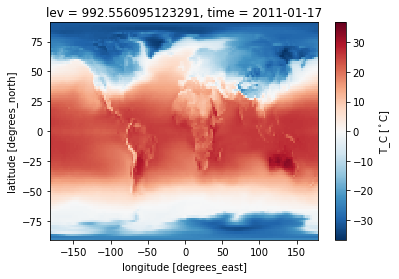
Notice how the labels use both the attribute “standard_name” and “units” from the dataset.
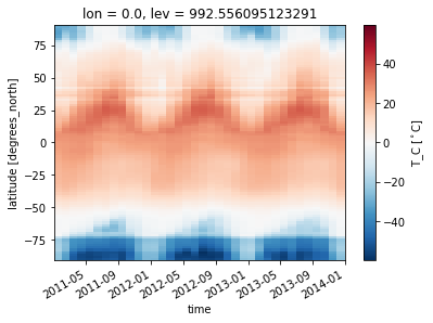
ds['T_C'].sel(lev=1000., lon=0, method='nearest').plot(x='time')
<matplotlib.collections.QuadMesh at 0x7fead9fc6430>
Slice:
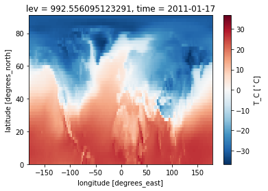
ds_s['T_C'].sel(lat=slice(0,90)).isel(time=0).plot()
<matplotlib.collections.QuadMesh at 0x7fead9f22ee0>
Super quick averaging etc
da_T = ds['T_C']
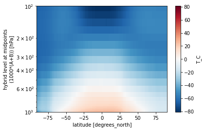
Mean:
da_T.mean(['time','lon']).plot(ylim=[1000,100], yscale='log')
<matplotlib.collections.QuadMesh at 0x7fead9e4cfd0>
Standard deviation
da_T.isel(lev=-1).std(['time']).plot()
<matplotlib.collections.QuadMesh at 0x7fead9d0e520>
Temperature change much stronger over land than ocean…
Seasonal average
month = (ds['time.month']==7) | (ds['time.month']==8)
ds_sum = ds.where(month).mean('time')
ds_sum
<xarray.Dataset>
Dimensions:  (lat: 96, lev: 32, lon: 144)
Coordinates:
  * lat      (lat) float64 -90.0 -88.11 -86.21 -84.32 ... 84.32 86.21 88.11 90.0
  * lon      (lon) float64 -180.0 -177.5 -175.0 -172.5 ... 172.5 175.0 177.5
  * lev      (lev) float64 3.643 7.595 14.36 24.61 ... 936.2 957.5 976.3 992.6
Data variables:
    hyam     (lev) float64 0.003643 0.007595 0.01436 ... 0.006255 0.001989 0.0
    hybm     (lev) float64 0.0 0.0 0.0 0.0 0.0 ... 0.9251 0.9512 0.9743 0.9926
    P0       float64 1e+05
    N_AER    (lev, lat, lon) float32 0.01799 0.01799 0.01799 ... 13.3 13.3 13.31
    PS       (lat, lon) float32 6.869e+04 6.869e+04 ... 1.012e+05 1.012e+05
    T        (lev, lat, lon) float32 202.9 202.9 202.9 ... 272.2 272.2 272.2
    U        (lev, lat, lon) float32 7.391 7.34 7.276 ... -0.4215 -0.394 -0.3657
    V        (lev, lat, lon) float32 1.004 1.325 1.644 ... 0.6221 0.6399 0.6565
T_C (lev, lat, lon) float32 -70.26 -70.26 -70.26 ... -0.9582 -0.9582- lat: 96
- lev: 32
- lon: 144
- lat(lat)float64-90.0 -88.11 -86.21 ... 88.11 90.0
- long_name :
- latitude
- units :
- degrees_north
array([-90. , -88.105263, -86.210526, -84.315789, -82.421053, -80.526316, -78.631579, -76.736842, -74.842105, -72.947368, -71.052632, -69.157895, -67.263158, -65.368421, -63.473684, -61.578947, -59.684211, -57.789474, -55.894737, -54. , -52.105263, -50.210526, -48.315789, -46.421053, -44.526316, -42.631579, -40.736842, -38.842105, -36.947368, -35.052632, -33.157895, -31.263158, -29.368421, -27.473684, -25.578947, -23.684211, -21.789474, -19.894737, -18. , -16.105263, -14.210526, -12.315789, -10.421053, -8.526316, -6.631579, -4.736842, -2.842105, -0.947368, 0.947368, 2.842105, 4.736842, 6.631579, 8.526316, 10.421053, 12.315789, 14.210526, 16.105263, 18. , 19.894737, 21.789474, 23.684211, 25.578947, 27.473684, 29.368421, 31.263158, 33.157895, 35.052632, 36.947368, 38.842105, 40.736842, 42.631579, 44.526316, 46.421053, 48.315789, 50.210526, 52.105263, 54. , 55.894737, 57.789474, 59.684211, 61.578947, 63.473684, 65.368421, 67.263158, 69.157895, 71.052632, 72.947368, 74.842105, 76.736842, 78.631579, 80.526316, 82.421053, 84.315789, 86.210526, 88.105263, 90. ]) - lon(lon)float64-180.0 -177.5 ... 175.0 177.5
- long_name :
- longitude
- units :
- degrees_east
array([-180. , -177.5, -175. , -172.5, -170. , -167.5, -165. , -162.5, -160. , -157.5, -155. , -152.5, -150. , -147.5, -145. , -142.5, -140. , -137.5, -135. , -132.5, -130. , -127.5, -125. , -122.5, -120. , -117.5, -115. , -112.5, -110. , -107.5, -105. , -102.5, -100. , -97.5, -95. , -92.5, -90. , -87.5, -85. , -82.5, -80. , -77.5, -75. , -72.5, -70. , -67.5, -65. , -62.5, -60. , -57.5, -55. , -52.5, -50. , -47.5, -45. , -42.5, -40. , -37.5, -35. , -32.5, -30. , -27.5, -25. , -22.5, -20. , -17.5, -15. , -12.5, -10. , -7.5, -5. , -2.5, 0. , 2.5, 5. , 7.5, 10. , 12.5, 15. , 17.5, 20. , 22.5, 25. , 27.5, 30. , 32.5, 35. , 37.5, 40. , 42.5, 45. , 47.5, 50. , 52.5, 55. , 57.5, 60. , 62.5, 65. , 67.5, 70. , 72.5, 75. , 77.5, 80. , 82.5, 85. , 87.5, 90. , 92.5, 95. , 97.5, 100. , 102.5, 105. , 107.5, 110. , 112.5, 115. , 117.5, 120. , 122.5, 125. , 127.5, 130. , 132.5, 135. , 137.5, 140. , 142.5, 145. , 147.5, 150. , 152.5, 155. , 157.5, 160. , 162.5, 165. , 167.5, 170. , 172.5, 175. , 177.5]) - lev(lev)float643.643 7.595 14.36 ... 976.3 992.6
- long_name :
- hybrid level at midpoints (1000*(A+B))
- units :
- hPa
- positive :
- down
- standard_name :
- atmosphere_hybrid_sigma_pressure_coordinate
- formula_terms :
- a: hyam b: hybm p0: P0 ps: PS
array([  3.643466,   7.59482 ,  14.356632,  24.61222 ,  35.92325 ,  43.19375 ,
        51.677499,  61.520498,  73.750958,  87.82123 , 103.317127, 121.547241,
       142.994039, 168.22508 , 197.908087, 232.828619, 273.910817, 322.241902,
       379.100904, 445.992574, 524.687175, 609.778695, 691.38943 , 763.404481,
       820.858369, 859.534767, 887.020249, 912.644547, 936.198398, 957.48548 ,
       976.325407, 992.556095])
- hyam(lev)float640.003643 0.007595 ... 0.001989 0.0
array([0.00364347, 0.00759482, 0.01435663, 0.02461222, 0.03592325, 0.04319375, 0.0516775 , 0.0615205 , 0.07375096, 0.08782123, 0.10331713, 0.12154724, 0.14299404, 0.16822508, 0.17823067, 0.17032433, 0.16102291, 0.15008029, 0.13720686, 0.12206194, 0.10424471, 0.08497915, 0.0665017 , 0.05019679, 0.03718866, 0.02843195, 0.02220898, 0.01640738, 0.01107456, 0.00625495, 0.00198941, 0. ]) - hybm(lev)float640.0 0.0 0.0 ... 0.9743 0.9926
array([0. , 0. , 0. , 0. , 0. , 0. , 0. , 0. , 0. , 0. , 0. , 0. , 0. , 0. , 0.01967741, 0.06250429, 0.11288791, 0.17216162, 0.24189404, 0.32393064, 0.42044246, 0.52479954, 0.62488773, 0.71320769, 0.78366971, 0.83110282, 0.86481127, 0.89623716, 0.92512384, 0.95123053, 0.974336 , 0.9925561 ]) - P0()float641e+05
array(100000.)
- N_AER(lev, lat, lon)float320.01799 0.01799 ... 13.3 13.31
array([[[1.7986173e-02, 1.7986173e-02, 1.7986173e-02, ..., 1.7986173e-02, 1.7986173e-02, 1.7986173e-02], [1.8111210e-02, 1.8107342e-02, 1.8103236e-02, ..., 1.8122591e-02, 1.8118849e-02, 1.8115008e-02], [1.8548474e-02, 1.8537238e-02, 1.8525066e-02, ..., 1.8575532e-02, 1.8567344e-02, 1.8558349e-02], ..., [5.9344987e-03, 5.9341914e-03, 5.9330747e-03, ..., 5.9329178e-03, 5.9334631e-03, 5.9341299e-03], [6.0512559e-03, 6.0493923e-03, 6.0474407e-03, ..., 6.0567441e-03, 6.0548573e-03, 6.0530514e-03], [6.0994383e-03, 6.0994383e-03, 6.0994383e-03, ..., 6.0994383e-03, 6.0994383e-03, 6.0994383e-03]], [[4.1006204e-02, 4.1006204e-02, 4.1006204e-02, ..., 4.1006204e-02, 4.1006204e-02, 4.1006204e-02], [4.1075446e-02, 4.1075800e-02, 4.1076310e-02, ..., 4.1074593e-02, 4.1074913e-02, 4.1075159e-02], [4.1167170e-02, 4.1174784e-02, 4.1182201e-02, ..., 4.1145105e-02, 4.1152228e-02, 4.1159671e-02], ... [3.7967278e+01, 3.8113823e+01, 3.8014065e+01, ..., 3.8805912e+01, 3.8918957e+01, 3.7824787e+01], [3.6096416e+01, 3.6029415e+01, 3.6020535e+01, ..., 3.6349751e+01, 3.6196239e+01, 3.6132069e+01], [3.5970768e+01, 3.5970566e+01, 3.5970737e+01, ..., 3.5968800e+01, 3.5968784e+01, 3.5969482e+01]], [[3.4683864e+00, 3.4684248e+00, 3.4684536e+00, ..., 3.4681842e+00, 3.4682109e+00, 3.4683325e+00], [3.5714447e+00, 3.5537269e+00, 3.5360434e+00, ..., 3.6024828e+00, 3.5886953e+00, 3.5803051e+00], [3.6493952e+00, 3.5949886e+00, 3.5358546e+00, ..., 3.8649702e+00, 3.8052540e+00, 3.7325652e+00], ..., [1.5509464e+01, 1.5511327e+01, 1.5274704e+01, ..., 1.5036141e+01, 1.5488576e+01, 1.5494289e+01], [1.4412013e+01, 1.4096001e+01, 1.4765851e+01, ..., 1.3413643e+01, 1.3525212e+01, 1.3559123e+01], [1.3306618e+01, 1.3306272e+01, 1.3306267e+01, ..., 1.3303113e+01, 1.3302909e+01, 1.3306339e+01]]], dtype=float32) - PS(lat, lon)float326.869e+04 6.869e+04 ... 1.012e+05
array([[ 68691.445, 68691.445, 68691.445, ..., 68691.445, 68691.445, 68691.445], [ 65252.918, 65339.844, 65429.51 , ..., 65186.99 , 65206.973, 65229.113], [ 67992.33 , 68332.375, 68734.69 , ..., 68218.125, 68108.945, 68035.336], ..., [101189.98 , 101181.27 , 101172.31 , ..., 101137.97 , 101156.98 , 101174.49 ], [101193.24 , 101197.18 , 101202.25 , ..., 101166.625, 101175.23 , 101184.15 ], [101179.414, 101179.414, 101179.414, ..., 101179.414, 101179.414, 101179.414]], dtype=float32) - T(lev, lat, lon)float32202.9 202.9 202.9 ... 272.2 272.2
array([[[202.88554, 202.88554, 202.88554, ..., 202.88554, 202.88554, 202.88554], [203.55504, 203.5473 , 203.53859, ..., 203.57164, 203.56715, 203.56158], [204.41087, 204.39752, 204.38304, ..., 204.43852, 204.43129, 204.42201], ..., [258.35306, 258.3522 , 258.35123, ..., 258.35458, 258.35422, 258.35376], [258.34116, 258.3401 , 258.339 , ..., 258.34387, 258.3431 , 258.34216], [258.3267 , 258.3267 , 258.3267 , ..., 258.3267 , 258.3267 , 258.3267 ]], [[197.07903, 197.07903, 197.07903, ..., 197.07903, 197.07903, 197.07903], [197.59735, 197.58258, 197.5673 , ..., 197.63637, 197.62402, 197.61101], [198.43327, 198.4046 , 198.37657, ..., 198.50781, 198.48463, 198.45964], ... [271.8259 , 271.81924, 271.8115 , ..., 271.78098, 271.79874, 271.8159 ], [271.6981 , 271.69827, 271.69815, ..., 271.6869 , 271.69193, 271.69626], [271.55237, 271.55237, 271.55237, ..., 271.55237, 271.55237, 271.55237]], [[220.01125, 220.0097 , 220.00868, ..., 220.01497, 220.01408, 220.01286], [219.98546, 220.08911, 220.18608, ..., 219.86116, 219.90332, 219.93648], [228.0412 , 228.78844, 229.26945, ..., 227.27507, 227.46887, 227.81172], ..., [272.40585, 272.3934 , 272.38065, ..., 272.38303, 272.39462, 272.40125], [272.31424, 272.31494, 272.31424, ..., 272.30652, 272.31018, 272.31326], [272.1918 , 272.1918 , 272.1918 , ..., 272.1918 , 272.1918 , 272.1918 ]]], dtype=float32) - U(lev, lat, lon)float327.391 7.34 7.276 ... -0.394 -0.3657
array([[[ 7.39123 , 7.3404026 , 7.275603 , ..., 7.45904 , 7.4506054 , 7.4279876 ], [14.479408 , 14.429122 , 14.361183 , ..., 14.522685 , 14.526362 , 14.51188 ], [20.258013 , 20.205286 , 20.132715 , ..., 20.292315 , 20.302294 , 20.290573 ], ..., [-1.1146437 , -1.1090753 , -1.1030668 , ..., -1.1274763 , -1.1239392 , -1.1196352 ], [-0.6215214 , -0.62102157, -0.620526 , ..., -0.62292975, -0.6224782 , -0.6220094 ], [ 0.03603012, 0.03560662, 0.0351153 , ..., 0.03688656, 0.03667071, 0.03638504]], [[ 5.530292 , 5.522363 , 5.503922 , ..., 5.490955 , 5.514572 , 5.5276933 ], [10.640478 , 10.624447 , 10.596233 , ..., 10.61387 , 10.635348 , 10.644154 ], [15.151515 , 15.128281 , 15.091004 , ..., 15.131355 , 15.153908 , 15.1603155 ], ... [-0.38241994, -0.37808958, -0.36921516, ..., -0.37270746, -0.3789377 , -0.38292608], [-0.3046574 , -0.27710113, -0.24971397, ..., -0.389061 , -0.36036468, -0.33236775], [-0.2897645 , -0.2522249 , -0.21420284, ..., -0.39879847, -0.36311814, -0.32675073]], [[ 3.7669709 , 3.4682417 , 3.1631877 , ..., 4.6178093 , 4.3424063 , 4.0586195 ], [-2.039138 , -2.0782287 , -2.111614 , ..., -1.8343946 , -1.9192523 , -1.9867474 ], [ 0.7380986 , 0.8664727 , 0.92238516, ..., 0.07377125, 0.3236346 , 0.55084825], ..., [-0.39446747, -0.39623132, -0.39381883, ..., -0.38285258, -0.38817003, -0.392043 ], [-0.39340416, -0.37519348, -0.35699585, ..., -0.45005608, -0.4303613 , -0.4118218 ], [-0.33668396, -0.30705747, -0.27684963, ..., -0.42148638, -0.39395377, -0.36565718]]], dtype=float32) - V(lev, lat, lon)float321.004 1.325 1.644 ... 0.6399 0.6565
array([[[ 1.00396347e+00, 1.32540894e+00, 1.64433134e+00, ..., 3.06254234e-02, 3.55954885e-01, 6.80607021e-01], [ 1.14025724e+00, 1.50571489e+00, 1.86828649e+00, ..., 3.59791107e-02, 4.04443055e-01, 7.72850931e-01], [ 7.88153589e-01, 1.17143297e+00, 1.55356824e+00, ..., -3.59685570e-01, 2.16981564e-02, 4.04614329e-01], ..., [ 2.23243032e-02, 3.08354702e-02, 3.85811329e-02, ..., -6.80489326e-03, 3.39241815e-03, 1.31411953e-02], [ 2.88868342e-02, 3.30834277e-02, 3.68954837e-02, ..., 1.44335926e-02, 1.95146110e-02, 2.43485663e-02], [-8.92307330e-03, -1.04861856e-02, -1.20293396e-02, ..., -4.14385414e-03, -5.74888801e-03, -7.34296441e-03]], [[ 6.10973053e-02, 3.02267194e-01, 5.42861581e-01, ..., -6.61273241e-01, -4.21131730e-01, -1.80188656e-01], [ 1.73292086e-01, 4.36991781e-01, 6.99402750e-01, ..., -6.19174302e-01, -3.55436236e-01, -9.10642967e-02], [ 4.23814468e-02, 3.16929460e-01, 5.91296315e-01, ..., -7.77750194e-01, -5.05434096e-01, -2.31889680e-01], ... 6.90535963e-01, 6.99401140e-01, 7.07436740e-01], [ 8.48888338e-01, 8.55763733e-01, 8.61199200e-01, ..., 8.23416889e-01, 8.33414376e-01, 8.42045069e-01], [ 8.54311407e-01, 8.66139412e-01, 8.76317024e-01, ..., 8.09178054e-01, 8.25804949e-01, 8.40860307e-01]], [[ 6.75157309e+00, 6.90882635e+00, 7.05307817e+00, ..., 6.20331764e+00, 6.39851904e+00, 6.58141184e+00], [ 8.60573864e+00, 8.68464565e+00, 8.75355816e+00, ..., 8.31920147e+00, 8.42445755e+00, 8.51937103e+00], [ 1.12631788e+01, 1.12480917e+01, 1.12178802e+01, ..., 1.11555176e+01, 1.12145271e+01, 1.12590971e+01], ..., [ 4.88537878e-01, 4.92254883e-01, 4.97978419e-01, ..., 4.74405676e-01, 4.79454309e-01, 4.83651519e-01], [ 6.48124695e-01, 6.57615721e-01, 6.65353119e-01, ..., 6.13545597e-01, 6.26336157e-01, 6.37737453e-01], [ 6.71818554e-01, 6.85864031e-01, 6.98605716e-01, ..., 6.22114539e-01, 6.39912307e-01, 6.56496942e-01]]], dtype=float32) - T_C(lev, lat, lon)float32-70.26 -70.26 ... -0.9582 -0.9582
array([[[-70.26444   , -70.26444   , -70.26444   , ..., -70.26444   ,
         -70.26444   , -70.26444   ],
        [-69.59496   , -69.6027    , -69.61139   , ..., -69.57836   ,
         -69.582825  , -69.5884    ],
        [-68.73913   , -68.752464  , -68.766945  , ..., -68.71149   ,
         -68.71871   , -68.727974  ],
        ...,
        [-14.796941  , -14.79778   , -14.798778  , ..., -14.795433  ,
         -14.795749  , -14.796257  ],
        [-14.808835  , -14.809901  , -14.811002  , ..., -14.806122  ,
         -14.806912  , -14.807823  ],
        [-14.8233    , -14.8233    , -14.8233    , ..., -14.8233    ,
         -14.8233    , -14.8233    ]],

       [[-76.07096   , -76.07096   , -76.07096   , ..., -76.07096   ,
         -76.07096   , -76.07096   ],
        [-75.552635  , -75.56742   , -75.58268   , ..., -75.51362   ,
         -75.52596   , -75.539     ],
        [-74.716736  , -74.74539   , -74.77344   , ..., -74.64219   ,
         -74.66537   , -74.69036   ],
...
        [ -1.3241018 ,  -1.3307596 ,  -1.3385111 , ...,  -1.3690186 ,
          -1.3512319 ,  -1.3341217 ],
        [ -1.4519043 ,  -1.451711  ,  -1.451828  , ...,  -1.4630991 ,
          -1.4580536 ,  -1.4537455 ],
        [ -1.597641  ,  -1.5976359 ,  -1.5976359 , ...,  -1.5976257 ,
          -1.5976206 ,  -1.5976359 ]],

       [[-53.138744  , -53.14029   , -53.141315  , ..., -53.135025  ,
         -53.135914  , -53.137127  ],
        [-53.16454   , -53.060883  , -52.96391   , ..., -53.288837  ,
         -53.246674  , -53.21352   ],
        [-45.10879   , -44.36156   , -43.880524  , ..., -45.87494   ,
         -45.681133  , -45.338276  ],
        ...,
        [ -0.7441762 ,  -0.7565715 ,  -0.76933795, ...,  -0.7669525 ,
          -0.7553609 ,  -0.74871826],
        [ -0.83573914,  -0.8350525 ,  -0.8357442 , ...,  -0.8434703 ,
          -0.83980817,  -0.83673096],
        [ -0.9582011 ,  -0.9582062 ,  -0.9582062 , ...,  -0.9582062 ,
          -0.9582062 ,  -0.9582062 ]]], dtype=float32)
ds_season = ds.groupby('time.season').mean()
ds_season
<xarray.Dataset>
Dimensions:  (lat: 96, lev: 32, lon: 144, season: 4)
Coordinates:
  * lat      (lat) float64 -90.0 -88.11 -86.21 -84.32 ... 84.32 86.21 88.11 90.0
  * lon      (lon) float64 -180.0 -177.5 -175.0 -172.5 ... 172.5 175.0 177.5
  * lev      (lev) float64 3.643 7.595 14.36 24.61 ... 936.2 957.5 976.3 992.6
  * season   (season) object 'DJF' 'JJA' 'MAM' 'SON'
Data variables:
    hyam     (season, lev) float64 0.003643 0.007595 0.01436 ... 0.001989 0.0
    hybm     (season, lev) float64 0.0 0.0 0.0 0.0 ... 0.9512 0.9743 0.9926
    P0       (season) float64 1e+05 1e+05 1e+05 1e+05
    N_AER    (season, lev, lat, lon) float32 0.006281 0.006281 ... 16.53 16.53
    PS       (season, lat, lon) float32 6.922e+04 6.922e+04 ... 1.011e+05
    T        (season, lev, lat, lon) float32 263.9 263.9 263.9 ... 259.2 259.2
    U        (season, lev, lat, lon) float32 0.6781 0.7017 ... 0.4854 0.5219
    V        (season, lev, lat, lon) float32 -0.5561 -0.526 ... 0.8473 0.8253
T_C (season, lev, lat, lon) float32 -9.245 -9.245 ... -13.91 -13.91- lat: 96
- lev: 32
- lon: 144
- season: 4
- lat(lat)float64-90.0 -88.11 -86.21 ... 88.11 90.0
- long_name :
- latitude
- units :
- degrees_north
array([-90. , -88.105263, -86.210526, -84.315789, -82.421053, -80.526316, -78.631579, -76.736842, -74.842105, -72.947368, -71.052632, -69.157895, -67.263158, -65.368421, -63.473684, -61.578947, -59.684211, -57.789474, -55.894737, -54. , -52.105263, -50.210526, -48.315789, -46.421053, -44.526316, -42.631579, -40.736842, -38.842105, -36.947368, -35.052632, -33.157895, -31.263158, -29.368421, -27.473684, -25.578947, -23.684211, -21.789474, -19.894737, -18. , -16.105263, -14.210526, -12.315789, -10.421053, -8.526316, -6.631579, -4.736842, -2.842105, -0.947368, 0.947368, 2.842105, 4.736842, 6.631579, 8.526316, 10.421053, 12.315789, 14.210526, 16.105263, 18. , 19.894737, 21.789474, 23.684211, 25.578947, 27.473684, 29.368421, 31.263158, 33.157895, 35.052632, 36.947368, 38.842105, 40.736842, 42.631579, 44.526316, 46.421053, 48.315789, 50.210526, 52.105263, 54. , 55.894737, 57.789474, 59.684211, 61.578947, 63.473684, 65.368421, 67.263158, 69.157895, 71.052632, 72.947368, 74.842105, 76.736842, 78.631579, 80.526316, 82.421053, 84.315789, 86.210526, 88.105263, 90. ]) - lon(lon)float64-180.0 -177.5 ... 175.0 177.5
- long_name :
- longitude
- units :
- degrees_east
array([-180. , -177.5, -175. , -172.5, -170. , -167.5, -165. , -162.5, -160. , -157.5, -155. , -152.5, -150. , -147.5, -145. , -142.5, -140. , -137.5, -135. , -132.5, -130. , -127.5, -125. , -122.5, -120. , -117.5, -115. , -112.5, -110. , -107.5, -105. , -102.5, -100. , -97.5, -95. , -92.5, -90. , -87.5, -85. , -82.5, -80. , -77.5, -75. , -72.5, -70. , -67.5, -65. , -62.5, -60. , -57.5, -55. , -52.5, -50. , -47.5, -45. , -42.5, -40. , -37.5, -35. , -32.5, -30. , -27.5, -25. , -22.5, -20. , -17.5, -15. , -12.5, -10. , -7.5, -5. , -2.5, 0. , 2.5, 5. , 7.5, 10. , 12.5, 15. , 17.5, 20. , 22.5, 25. , 27.5, 30. , 32.5, 35. , 37.5, 40. , 42.5, 45. , 47.5, 50. , 52.5, 55. , 57.5, 60. , 62.5, 65. , 67.5, 70. , 72.5, 75. , 77.5, 80. , 82.5, 85. , 87.5, 90. , 92.5, 95. , 97.5, 100. , 102.5, 105. , 107.5, 110. , 112.5, 115. , 117.5, 120. , 122.5, 125. , 127.5, 130. , 132.5, 135. , 137.5, 140. , 142.5, 145. , 147.5, 150. , 152.5, 155. , 157.5, 160. , 162.5, 165. , 167.5, 170. , 172.5, 175. , 177.5]) - lev(lev)float643.643 7.595 14.36 ... 976.3 992.6
- long_name :
- hybrid level at midpoints (1000*(A+B))
- units :
- hPa
- positive :
- down
- standard_name :
- atmosphere_hybrid_sigma_pressure_coordinate
- formula_terms :
- a: hyam b: hybm p0: P0 ps: PS
array([ 3.643466, 7.59482 , 14.356632, 24.61222 , 35.92325 , 43.19375 , 51.677499, 61.520498, 73.750958, 87.82123 , 103.317127, 121.547241, 142.994039, 168.22508 , 197.908087, 232.828619, 273.910817, 322.241902, 379.100904, 445.992574, 524.687175, 609.778695, 691.38943 , 763.404481, 820.858369, 859.534767, 887.020249, 912.644547, 936.198398, 957.48548 , 976.325407, 992.556095]) - season(season)object'DJF' 'JJA' 'MAM' 'SON'
array(['DJF', 'JJA', 'MAM', 'SON'], dtype=object)
- hyam(season, lev)float640.003643 0.007595 ... 0.001989 0.0
array([[0.00364347, 0.00759482, 0.01435663, 0.02461222, 0.03592325, 0.04319375, 0.0516775 , 0.0615205 , 0.07375096, 0.08782123, 0.10331713, 0.12154724, 0.14299404, 0.16822508, 0.17823067, 0.17032433, 0.16102291, 0.15008029, 0.13720686, 0.12206194, 0.10424471, 0.08497915, 0.0665017 , 0.05019679, 0.03718866, 0.02843195, 0.02220898, 0.01640738, 0.01107456, 0.00625495, 0.00198941, 0. ], [0.00364347, 0.00759482, 0.01435663, 0.02461222, 0.03592325, 0.04319375, 0.0516775 , 0.0615205 , 0.07375096, 0.08782123, 0.10331713, 0.12154724, 0.14299404, 0.16822508, 0.17823067, 0.17032433, 0.16102291, 0.15008029, 0.13720686, 0.12206194, 0.10424471, 0.08497915, 0.0665017 , 0.05019679, 0.03718866, 0.02843195, 0.02220898, 0.01640738, 0.01107456, 0.00625495, 0.00198941, 0. ], [0.00364347, 0.00759482, 0.01435663, 0.02461222, 0.03592325, 0.04319375, 0.0516775 , 0.0615205 , 0.07375096, 0.08782123, 0.10331713, 0.12154724, 0.14299404, 0.16822508, 0.17823067, 0.17032433, 0.16102291, 0.15008029, 0.13720686, 0.12206194, 0.10424471, 0.08497915, 0.0665017 , 0.05019679, 0.03718866, 0.02843195, 0.02220898, 0.01640738, 0.01107456, 0.00625495, 0.00198941, 0. ], [0.00364347, 0.00759482, 0.01435663, 0.02461222, 0.03592325, 0.04319375, 0.0516775 , 0.0615205 , 0.07375096, 0.08782123, 0.10331713, 0.12154724, 0.14299404, 0.16822508, 0.17823067, 0.17032433, 0.16102291, 0.15008029, 0.13720686, 0.12206194, 0.10424471, 0.08497915, 0.0665017 , 0.05019679, 0.03718866, 0.02843195, 0.02220898, 0.01640738, 0.01107456, 0.00625495, 0.00198941, 0. ]]) - hybm(season, lev)float640.0 0.0 0.0 ... 0.9743 0.9926
array([[0. , 0. , 0. , 0. , 0. , 0. , 0. , 0. , 0. , 0. , 0. , 0. , 0. , 0. , 0.01967741, 0.06250429, 0.11288791, 0.17216162, 0.24189404, 0.32393064, 0.42044246, 0.52479954, 0.62488773, 0.71320769, 0.78366971, 0.83110282, 0.86481127, 0.89623716, 0.92512384, 0.95123053, 0.974336 , 0.9925561 ], [0. , 0. , 0. , 0. , 0. , 0. , 0. , 0. , 0. , 0. , 0. , 0. , 0. , 0. , 0.01967741, 0.06250429, 0.11288791, 0.17216162, 0.24189404, 0.32393064, 0.42044246, 0.52479954, 0.62488773, 0.71320769, 0.78366971, 0.83110282, 0.86481127, 0.89623716, 0.92512384, 0.95123053, 0.974336 , 0.9925561 ], [0. , 0. , 0. , 0. , 0. , 0. , 0. , 0. , 0. , 0. , 0. , 0. , 0. , 0. , 0.01967741, 0.06250429, 0.11288791, 0.17216162, 0.24189404, 0.32393064, 0.42044246, 0.52479954, 0.62488773, 0.71320769, 0.78366971, 0.83110282, 0.86481127, 0.89623716, 0.92512384, 0.95123053, 0.974336 , 0.9925561 ], [0. , 0. , 0. , 0. , 0. , 0. , 0. , 0. , 0. , 0. , 0. , 0. , 0. , 0. , 0.01967741, 0.06250429, 0.11288791, 0.17216162, 0.24189404, 0.32393064, 0.42044246, 0.52479954, 0.62488773, 0.71320769, 0.78366971, 0.83110282, 0.86481127, 0.89623716, 0.92512384, 0.95123053, 0.974336 , 0.9925561 ]]) - P0(season)float641e+05 1e+05 1e+05 1e+05
array([100000., 100000., 100000., 100000.])
- N_AER(season, lev, lat, lon)float320.006281 0.006281 ... 16.53 16.53
array([[[[6.28054794e-03, 6.28054794e-03, 6.28054794e-03, ..., 6.28054794e-03, 6.28054794e-03, 6.28054794e-03], [6.31130813e-03, 6.30999682e-03, 6.30854256e-03, ..., 6.31437358e-03, 6.31345715e-03, 6.31246716e-03], [6.35629287e-03, 6.35398505e-03, 6.35069190e-03, ..., 6.36250759e-03, 6.36028778e-03, 6.35822956e-03], ..., [4.03482020e-02, 4.03706543e-02, 4.03931364e-02, ..., 4.02851999e-02, 4.03077751e-02, 4.03273553e-02], [3.93667631e-02, 3.93775105e-02, 3.93860862e-02, ..., 3.93066145e-02, 3.93263251e-02, 3.93496007e-02], [3.83674316e-02, 3.83674316e-02, 3.83674316e-02, ..., 3.83674316e-02, 3.83674316e-02, 3.83674316e-02]], [[6.86971247e-02, 6.86971247e-02, 6.86971247e-02, ..., 6.86971247e-02, 6.86971247e-02, 6.86971247e-02], [6.91883042e-02, 6.91581964e-02, 6.91256225e-02, ..., 6.92559034e-02, 6.92377537e-02, 6.92151934e-02], [6.97361976e-02, 6.96922839e-02, 6.96431249e-02, ..., 6.98694810e-02, 6.98314831e-02, 6.97820410e-02], ... 2.72275677e+01, 2.60849609e+01, 2.51911621e+01], [2.58603992e+01, 2.54049892e+01, 2.49414692e+01, ..., 2.69397659e+01, 2.66668148e+01, 2.63382816e+01], [2.77304306e+01, 2.77392521e+01, 2.77301273e+01, ..., 2.77303867e+01, 2.77295303e+01, 2.77294025e+01]], [[1.07460632e+01, 1.07460909e+01, 1.07461691e+01, ..., 1.07458162e+01, 1.07459221e+01, 1.07460127e+01], [9.94326401e+00, 9.87798691e+00, 9.81807423e+00, ..., 1.02882328e+01, 1.01789417e+01, 1.00537405e+01], [1.01583719e+01, 1.01861677e+01, 1.01585531e+01, ..., 1.04374828e+01, 1.03314552e+01, 1.02295408e+01], ..., [1.92233353e+01, 1.93865585e+01, 1.90421066e+01, ..., 2.02667561e+01, 1.97197742e+01, 1.96469097e+01], [1.76463490e+01, 1.74683781e+01, 1.73526993e+01, ..., 1.82269859e+01, 1.80763931e+01, 1.77846298e+01], [1.65312252e+01, 1.65311375e+01, 1.65317554e+01, ..., 1.65312595e+01, 1.65316391e+01, 1.65314751e+01]]]], dtype=float32) - PS(season, lat, lon)float326.922e+04 6.922e+04 ... 1.011e+05
array([[[ 69218.766, 69218.766, 69218.766, ..., 69218.766, 69218.766, 69218.766], [ 66037.664, 66121.414, 66207.93 , ..., 65974.27 , 65993.86 , 66015.03 ], [ 68854.56 , 69186.84 , 69579.92 , ..., 69070.586, 68966.84 , 68896.305], ..., [101846.25 , 101829.28 , 101811. , ..., 101806.36 , 101822.266, 101835.75 ], [101639.21 , 101637.71 , 101637.04 , ..., 101624.266, 101629.41 , 101634.48 ], [101451.94 , 101451.94 , 101451.94 , ..., 101451.94 , 101451.94 , 101451.94 ]], [[ 68789.375, 68789.375, 68789.375, ..., 68789.375, 68789.375, 68789.375], [ 65365.383, 65452.105, 65541.59 , ..., 65299.92 , 65319.82 , 65341.793], [ 68122.484, 68461.71 , 68863.38 , ..., 68352.12 , 68241.92 , 68167.016], ... [101956.305, 101950.28 , 101943.375, ..., 101889.78 , 101913.91 , 101936.39 ], [101852.66 , 101857.76 , 101863.49 , ..., 101819.266, 101830.21 , 101841.445], [101746.375, 101746.375, 101746.375, ..., 101746.375, 101746.375, 101746.375]], [[ 68881.086, 68881.086, 68881.086, ..., 68881.086, 68881.086, 68881.086], [ 65560.11 , 65645.945, 65734.47 , ..., 65494.223, 65514.445, 65536.53 ], [ 68307.875, 68640.586, 69035.625, ..., 68545.54 , 68432.97 , 68355.39 ], ..., [101194.82 , 101182.414, 101169.41 , ..., 101148.66 , 101165.93 , 101181.59 ], [101120.58 , 101123.29 , 101127.05 , ..., 101095.625, 101103.836, 101112.21 ], [101051.586, 101051.586, 101051.586, ..., 101051.586, 101051.586, 101051.586]]], dtype=float32) - T(season, lev, lat, lon)float32263.9 263.9 263.9 ... 259.2 259.2
array([[[[263.90543, 263.90543, 263.90543, ..., 263.90543, 263.90543, 263.90543], [263.8293 , 263.8299 , 263.83066, ..., 263.82828, 263.8285 , 263.82883], [263.73718, 263.7372 , 263.73822, ..., 263.7387 , 263.73822, 263.7376 ], ..., [220.39774, 220.38452, 220.36864, ..., 220.42035, 220.41582, 220.40823], [219.74033, 219.73405, 219.72614, ..., 219.74886, 219.74777, 219.74489], [218.6981 , 218.6981 , 218.6981 , ..., 218.6981 , 218.6981 , 218.6981 ]], [[246.1779 , 246.1779 , 246.1779 , ..., 246.1779 , 246.1779 , 246.1779 ], [246.07938, 246.07764, 246.07628, ..., 246.08504, 246.08298, 246.08109], [245.9385 , 245.93115, 245.926 , ..., 245.96066, 245.95367, 245.94615], ... [260.51602, 260.47867, 260.44138, ..., 260.55115, 260.54172, 260.5309 ], [260.453 , 260.43076, 260.40894, ..., 260.4902 , 260.48056, 260.46906], [260.28268, 260.28268, 260.28268, ..., 260.28268, 260.28268, 260.28268]], [[228.56093, 228.5593 , 228.55824, ..., 228.56477, 228.56386, 228.5626 ], [227.3517 , 227.43579, 227.5136 , ..., 227.326 , 227.33218, 227.33049], [233.6447 , 234.25388, 234.66417, ..., 233.26782, 233.3306 , 233.5293 ], ..., [260.02112, 259.98703, 259.9537 , ..., 260.10095, 260.075 , 260.047 ], [259.90082, 259.87448, 259.84515, ..., 259.96072, 259.94168, 259.92053], [259.24106, 259.2409 , 259.2411 , ..., 259.2411 , 259.2411 , 259.24106]]]], dtype=float32) - U(season, lev, lat, lon)float320.6781 0.7017 ... 0.4854 0.5219
array([[[[ 6.78081512e-01, 7.01694489e-01, 7.23971784e-01, ..., 5.99690080e-01, 6.27030730e-01, 6.53177738e-01], [-1.41270822e-02, 3.69813715e-05, 1.16184689e-02, ..., -7.29624033e-02, -5.05819768e-02, -3.09799835e-02], [-3.79267514e-01, -3.74312222e-01, -3.72618347e-01, ..., -4.16908741e-01, -4.00227487e-01, -3.87805104e-01], ..., [ 4.02558136e+01, 4.05386238e+01, 4.07433891e+01, ..., 3.89494209e+01, 3.94599609e+01, 3.98958778e+01], [ 3.63207817e+01, 3.65878487e+01, 3.67830963e+01, ..., 3.50967102e+01, 3.55742188e+01, 3.59826012e+01], [ 3.15966320e+01, 3.18394089e+01, 3.20215874e+01, ..., 3.05098362e+01, 3.09312096e+01, 3.12937088e+01]], [[ 1.31565964e+00, 1.34490371e+00, 1.37158751e+00, ..., 1.21314740e+00, 1.24971867e+00, 1.28391123e+00], [ 7.08594918e-01, 7.27423906e-01, 7.42690504e-01, ..., 6.30357504e-01, 6.60093546e-01, 6.86163664e-01], [ 5.59591353e-01, 5.66815436e-01, 5.69931269e-01, ..., 5.09791136e-01, 5.31516612e-01, 5.47946990e-01], ... 1.80565941e+00, 1.81366265e+00, 1.81684768e+00], [ 1.40761518e+00, 1.40596306e+00, 1.40300083e+00, ..., 1.39898825e+00, 1.40463710e+00, 1.40720773e+00], [ 1.17194080e+00, 1.19742417e+00, 1.22053444e+00, ..., 1.08245516e+00, 1.11442411e+00, 1.14427590e+00]], [[ 3.66142654e+00, 3.37230015e+00, 3.07690382e+00, ..., 4.48468733e+00, 4.21819448e+00, 3.94361377e+00], [-1.43481171e+00, -1.50281167e+00, -1.56427848e+00, ..., -1.14662600e+00, -1.25810599e+00, -1.35390532e+00], [ 7.18930185e-01, 8.00812364e-01, 8.22696090e-01, ..., 2.58407891e-01, 4.33471978e-01, 5.91223419e-01], ..., [ 1.09778368e+00, 1.11450720e+00, 1.12638485e+00, ..., 1.03337753e+00, 1.05724919e+00, 1.07942331e+00], [ 8.41345191e-01, 8.57699633e-01, 8.73181045e-01, ..., 7.80183971e-01, 8.03160131e-01, 8.23836088e-01], [ 5.57490528e-01, 5.91812193e-01, 6.25225782e-01, ..., 4.48015094e-01, 4.85435545e-01, 5.21936953e-01]]]], dtype=float32) - V(season, lev, lat, lon)float32-0.5561 -0.526 ... 0.8473 0.8253
array([[[[-5.56136489e-01, -5.26029706e-01, -4.94921565e-01, ..., -6.39886081e-01, -6.13119006e-01, -5.85184753e-01], [-3.42947036e-01, -3.11034948e-01, -2.79641986e-01, ..., -4.40846562e-01, -4.07957315e-01, -3.75287920e-01], [-4.11141068e-01, -3.77061188e-01, -3.42111498e-01, ..., -5.09337723e-01, -4.77156967e-01, -4.44464207e-01], ..., [ 6.23332548e+00, 4.66842318e+00, 3.09143472e+00, ..., 1.08159876e+01, 9.31103992e+00, 7.78218079e+00], [ 6.30383396e+00, 4.81863594e+00, 3.32256603e+00, ..., 1.06618767e+01, 9.22868633e+00, 7.77493286e+00], [ 6.25531960e+00, 4.87114048e+00, 3.47768760e+00, ..., 1.03259926e+01, 8.98534489e+00, 7.62759209e+00]], [[-6.99144185e-01, -6.41090572e-01, -5.81816494e-01, ..., -8.64891052e-01, -8.11151087e-01, -7.55867124e-01], [-4.83293176e-01, -4.25263733e-01, -3.67656887e-01, ..., -6.58610880e-01, -6.00107074e-01, -5.41619539e-01], [-5.37314534e-01, -4.77329463e-01, -4.16498810e-01, ..., -7.12978244e-01, -6.55059397e-01, -5.96528471e-01], ... 5.40717781e-01, 4.81030047e-01, 4.24284577e-01], [ 2.91965932e-01, 2.43409842e-01, 1.95463866e-01, ..., 4.43881810e-01, 3.92452151e-01, 3.41766506e-01], [ 6.08756721e-01, 5.57064056e-01, 5.04299045e-01, ..., 7.56516218e-01, 7.08580971e-01, 6.59298778e-01]], [[ 6.53891754e+00, 6.69210672e+00, 6.83256912e+00, ..., 6.00557137e+00, 6.19532108e+00, 6.37323427e+00], [ 8.32867241e+00, 8.41625118e+00, 8.49312019e+00, ..., 8.01074696e+00, 8.12822247e+00, 8.23384857e+00], [ 1.04156504e+01, 1.03486490e+01, 1.02690392e+01, ..., 1.04794607e+01, 1.04832964e+01, 1.04701958e+01], ..., [ 5.81824422e-01, 5.52566767e-01, 5.28445005e-01, ..., 6.74269140e-01, 6.42398715e-01, 6.11732602e-01], [ 5.96474409e-01, 5.71163297e-01, 5.45834780e-01, ..., 6.70256615e-01, 6.46387756e-01, 6.21220648e-01], [ 8.01786721e-01, 7.76694536e-01, 7.50134587e-01, ..., 8.67683947e-01, 8.47335517e-01, 8.25345278e-01]]]], dtype=float32) - T_C(season, lev, lat, lon)float32-9.245 -9.245 ... -13.91 -13.91
array([[[[ -9.244573  ,  -9.244573  ,  -9.244573  , ...,  -9.244573  ,
           -9.244573  ,  -9.244573  ],
         [ -9.320689  ,  -9.320112  ,  -9.3193445 , ...,  -9.321701  ,
           -9.321492  ,  -9.321158  ],
         [ -9.412844  ,  -9.412742  ,  -9.411798  , ...,  -9.411277  ,
           -9.4117775 ,  -9.41238   ],
         ...,
         [-52.75227   , -52.765465  , -52.78137   , ..., -52.72964   ,
          -52.734173  , -52.74176   ],
         [-53.40968   , -53.41594   , -53.423862  , ..., -53.401142  ,
          -53.40224   , -53.40509   ],
         [-54.45189   , -54.45189   , -54.45189   , ..., -54.45189   ,
          -54.45189   , -54.45189   ]],

        [[-26.97211   , -26.97211   , -26.97211   , ..., -26.97211   ,
          -26.97211   , -26.97211   ],
         [-27.070625  , -27.072344  , -27.073723  , ..., -27.064968  ,
          -27.067019  , -27.068897  ],
         [-27.211487  , -27.21885   , -27.224003  , ..., -27.18932   ,
          -27.196318  , -27.203846  ],
...
         [-12.633948  , -12.671317  , -12.7086115 , ..., -12.598827  ,
          -12.608288  , -12.619064  ],
         [-12.696964  , -12.719255  , -12.741072  , ..., -12.659801  ,
          -12.669423  , -12.680959  ],
         [-12.867314  , -12.8673315 , -12.867318  , ..., -12.867314  ,
          -12.867313  , -12.867318  ]],

        [[-44.589073  , -44.590687  , -44.591736  , ..., -44.58521   ,
          -44.586136  , -44.587387  ],
         [-45.79829   , -45.714207  , -45.636406  , ..., -45.823975  ,
          -45.817825  , -45.819515  ],
         [-39.505306  , -38.896107  , -38.48584   , ..., -39.882156  ,
          -39.819397  , -39.62071   ],
         ...,
         [-13.128864  , -13.162955  , -13.196298  , ..., -13.049055  ,
          -13.074986  , -13.103021  ],
         [-13.249176  , -13.275521  , -13.304836  , ..., -13.18929   ,
          -13.20833   , -13.2294655 ],
         [-13.908929  , -13.90906   , -13.908914  , ..., -13.908929  ,
          -13.908932  , -13.908949  ]]]], dtype=float32)
ds_season['T_C'].isel(lev=-1).plot(col='season')
<xarray.plot.facetgrid.FacetGrid at 0x7fead9cac040>
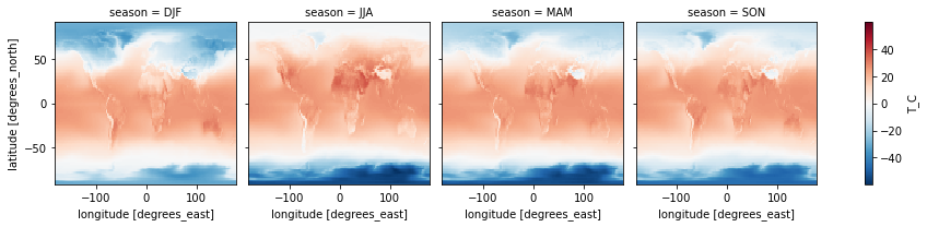
Controle the plot visuals:
# lets plot the wind fields
_ds = ds_s[['V','U']]
_da = np.sqrt(_ds['V']**2 + _ds['U']**2)

#_da.attrs['long_name'] = 'Wind speed'
#_da.attrs['units'] = 'm/s'
f,ax = plt.subplots(dpi=100)
_dm = _da.isel(time=0)
_dm.plot(cmap = plt.get_cmap('Reds'),ax=ax,
                   cbar_kwargs={'label':'Wind Speed [m/s]'})


_ds = ds_s.isel(time=0,lon =slice(0,None,2), lat=slice(0,None,2))
ax.quiver(_ds['lon'],_ds['lat'],_ds['U'],_ds['V'], scale=300, )

#ax.set_title('Wind strength and pattern')
#ax.set_xlabel('Longitude [$^\circ$E]')
<matplotlib.quiver.Quiver at 0x7fead9dc7fd0>
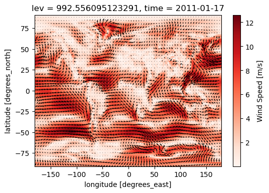
Plotting with cartopy
import cartopy as cy
import cartopy.crs as ccrs
f,ax = plt.subplots(dpi=100,subplot_kw={'projection':ccrs.PlateCarree()})


_dm.plot.pcolormesh(
    cmap = plt.get_cmap('Reds'),ax=ax,
    cbar_kwargs={
        'label':'Wind Speed [m/s]',
        'orientation':'horizontal',

    },
    transform=ccrs.PlateCarree(),
    x='lon',y='lat',
    levels = 6
)
ax.set_title('ilev:0; Mean over Time')
ax.coastlines()

gl = ax.gridlines(draw_labels=True)
gl.xlabels_top = False
gl.ylabels_right = False

ax.add_feature(cy.feature.BORDERS);
/opt/conda/lib/python3.8/site-packages/cartopy/mpl/gridliner.py:307: UserWarning: The .xlabels_top attribute is deprecated. Please use .top_labels to toggle visibility instead.
  warnings.warn('The .xlabels_top attribute is deprecated. Please '
/opt/conda/lib/python3.8/site-packages/cartopy/mpl/gridliner.py:343: UserWarning: The .ylabels_right attribute is deprecated. Please use .right_labels to toggle visibility instead.
  warnings.warn('The .ylabels_right attribute is deprecated. Please '
/opt/conda/lib/python3.8/site-packages/cartopy/io/__init__.py:260: DownloadWarning: Downloading: https://naciscdn.org/naturalearth/110m/cultural/ne_110m_admin_0_boundary_lines_land.zip
  warnings.warn('Downloading: {}'.format(url), DownloadWarning)
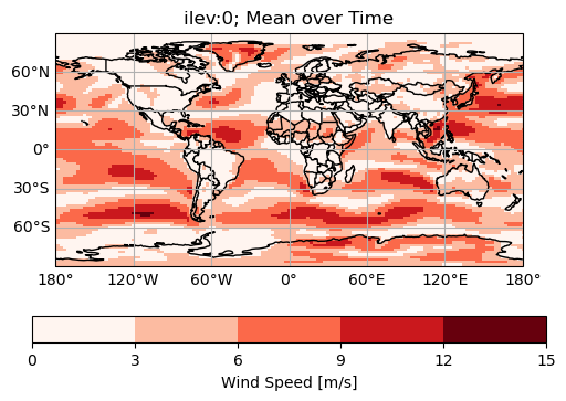
Convert to pandas & do some random fun stuff:
Maybe we e.g. want to compare with a station, or just use some of the considerable functionalities available from pandas. It’s easy to convert back and forth between xarray and pandas:
Pick out station:
Lets pick out Tjärnö research station!
lat_tjarno = 58.9
lon_tjarno = 11.1
# pick out surface
ds_surf =ds.isel(lev=-1)
ds_tjarno = ds_surf.sel(lat=lat_tjarno, lon = lon_tjarno, method ='nearest')
Resample:
df_tjarno = ds_tjarno.to_dataframe()
df_tjarno.head()
| lat | lon | lev | hyam | hybm | P0 | N_AER | PS | T | U | V | T_C | |
|---|---|---|---|---|---|---|---|---|---|---|---|---|
| time | ||||||||||||
| 2011-01-17 | 59.684211 | 10.0 | 992.556095 | 0.0 | 0.992556 | 100000.0 | 708.058899 | 96880.921875 | 269.207245 | 1.728664 | 0.475478 | -3.942749 |
| 2011-02-14 | 59.684211 | 10.0 | 992.556095 | 0.0 | 0.992556 | 100000.0 | 830.089844 | 97367.218750 | 266.607880 | -0.424161 | 1.017061 | -6.542114 |
| 2011-03-17 | 59.684211 | 10.0 | 992.556095 | 0.0 | 0.992556 | 100000.0 | 585.032104 | 97448.093750 | 271.787231 | 2.352789 | 0.320621 | -1.362762 |
| 2011-04-16 | 59.684211 | 10.0 | 992.556095 | 0.0 | 0.992556 | 100000.0 | 906.228210 | 97496.757812 | 279.498474 | 1.632975 | -0.223941 | 6.348480 |
| 2011-05-17 | 59.684211 | 10.0 | 992.556095 | 0.0 | 0.992556 | 100000.0 | 872.936096 | 97293.382812 | 281.770081 | 1.449824 | 1.465539 | 8.620087 |
df_yearly = df_tjarno.resample('Y' ).mean()#.plot()
df_yearly[['U','V']].plot()
<AxesSubplot:xlabel='time'>
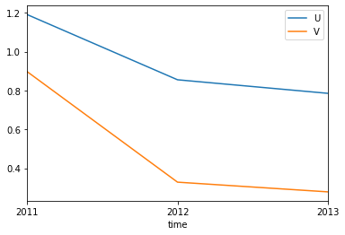
Using pandas specific tools:
ds_s['Wind_speed'] = np.sqrt(ds_s['U']**2 + ds_s['V']**2)
df = ds_s.to_dataframe()
df.head()
| lev | hyam | hybm | P0 | N_AER | PS | T | U | V | T_C | Wind_speed | |||
|---|---|---|---|---|---|---|---|---|---|---|---|---|---|
| lat | lon | time | |||||||||||
| -90.0 | -180.0 | 2011-01-17 | 992.556095 | 0.0 | 0.992556 | 100000.0 | 29.523746 | 69700.375000 | 249.113022 | 1.537032 | 4.258970 | -24.036972 | 4.527835 |
| 2011-02-14 | 992.556095 | 0.0 | 0.992556 | 100000.0 | 44.145832 | 69311.914062 | 239.829407 | 2.053496 | 4.899427 | -33.320587 | 5.312366 | ||
| 2011-03-17 | 992.556095 | 0.0 | 0.992556 | 100000.0 | 21.503481 | 68972.187500 | 223.339386 | 4.478918 | 5.187434 | -49.810608 | 6.853479 | ||
| 2011-04-16 | 992.556095 | 0.0 | 0.992556 | 100000.0 | 7.794546 | 68879.500000 | 219.738770 | 4.953977 | 5.242508 | -53.411224 | 7.212889 | ||
| 2011-05-17 | 992.556095 | 0.0 | 0.992556 | 100000.0 | 2.681895 | 68319.210938 | 218.717712 | 4.364126 | 5.071507 | -54.432281 | 6.690724 |
df[['U','V']].plot.hist(alpha=0.5, bins=200)
<AxesSubplot:ylabel='Frequency'>
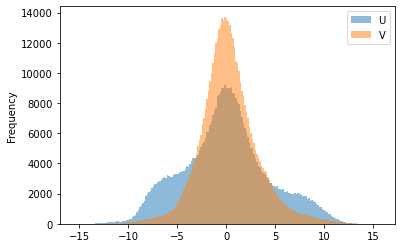
df_ri = df.reset_index()
df_ri.head()
| lat | lon | time | lev | hyam | hybm | P0 | N_AER | PS | T | U | V | T_C | Wind_speed | |
|---|---|---|---|---|---|---|---|---|---|---|---|---|---|---|
| 0 | -90.0 | -180.0 | 2011-01-17 | 992.556095 | 0.0 | 0.992556 | 100000.0 | 29.523746 | 69700.375000 | 249.113022 | 1.537032 | 4.258970 | -24.036972 | 4.527835 |
| 1 | -90.0 | -180.0 | 2011-02-14 | 992.556095 | 0.0 | 0.992556 | 100000.0 | 44.145832 | 69311.914062 | 239.829407 | 2.053496 | 4.899427 | -33.320587 | 5.312366 |
| 2 | -90.0 | -180.0 | 2011-03-17 | 992.556095 | 0.0 | 0.992556 | 100000.0 | 21.503481 | 68972.187500 | 223.339386 | 4.478918 | 5.187434 | -49.810608 | 6.853479 |
| 3 | -90.0 | -180.0 | 2011-04-16 | 992.556095 | 0.0 | 0.992556 | 100000.0 | 7.794546 | 68879.500000 | 219.738770 | 4.953977 | 5.242508 | -53.411224 | 7.212889 |
| 4 | -90.0 | -180.0 | 2011-05-17 | 992.556095 | 0.0 | 0.992556 | 100000.0 | 2.681895 | 68319.210938 | 218.717712 | 4.364126 | 5.071507 | -54.432281 | 6.690724 |
Check out the tradewinds (skip in presentation):
trops = (-20<df_ri['lat']) & (df_ri['lat']<20)
df_ri[['U','V']][trops].plot.hist(alpha=0.5, bins=200)
<AxesSubplot:ylabel='Frequency'>
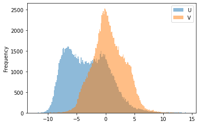
lets do something unnecesarily complicated :D
qcut, cut
qcut splits the data into quantile ranges
df_ri['wind_speed_cat'] = pd.qcut(df_ri['Wind_speed'],
                                  q=[0.05,0.17, 0.34,0.66, 0.83,0.95],
                                  labels=['very low','low','med','high','very high'])
Cut cuts into categories
df_ri['lat_cat'] = pd.cut(df_ri['lat'], [-90,-60,-30,0,30,60,90],
                          labels=['S polar','S mid','S tropics', 'N tropic', 'N mid','N polar'])
df_ri.groupby('lat_cat').mean()
| lat | lon | lev | hyam | hybm | P0 | N_AER | PS | T | U | V | T_C | Wind_speed | |
|---|---|---|---|---|---|---|---|---|---|---|---|---|---|
| lat_cat | |||||||||||||
| S polar | -74.842105 | -1.25 | 992.556095 | 0.0 | 0.992556 | 100000.0 | 37.134502 | 84496.015625 | 247.586441 | -0.925003 | 1.516052 | -25.563553 | 6.033710 |
| S mid | -45.473684 | -1.25 | 992.556095 | 0.0 | 0.992556 | 100000.0 | 244.884354 | 100566.250000 | 281.765289 | 5.021757 | -0.741656 | 8.615295 | 5.929924 |
| S tropics | -15.157895 | -1.25 | 992.556095 | 0.0 | 0.992556 | 100000.0 | 913.148193 | 99746.179688 | 295.955811 | -3.451257 | 1.499390 | 22.805801 | 4.714082 |
| N tropic | 15.157895 | -1.25 | 992.556095 | 0.0 | 0.992556 | 100000.0 | 1587.196167 | 99328.976562 | 297.289948 | -2.338687 | -0.537982 | 24.139965 | 4.485467 |
| N mid | 45.473684 | -1.25 | 992.556095 | 0.0 | 0.992556 | 100000.0 | 1425.352539 | 97057.734375 | 281.913513 | 1.253338 | 0.129856 | 8.763531 | 2.898627 |
| N polar | 75.789474 | -1.25 | 992.556095 | 0.0 | 0.992556 | 100000.0 | 225.529175 | 98979.195312 | 262.373474 | 0.150430 | -0.033408 | -10.776512 | 2.685246 |
sns.boxenplot(x="lat_cat", y="U",
              color="b",
              scale="linear", data=df_ri)
<AxesSubplot:xlabel='lat_cat', ylabel='U'>
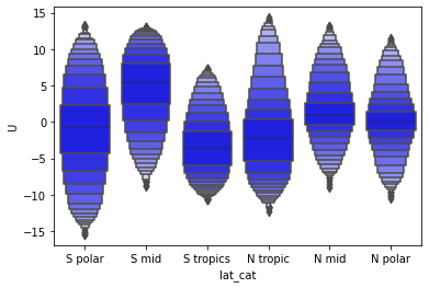
sns.boxenplot(x="wind_speed_cat", y="N_AER",
              color="b",
              scale="linear", data=df_ri,
             )
<AxesSubplot:xlabel='wind_speed_cat', ylabel='N_AER'>
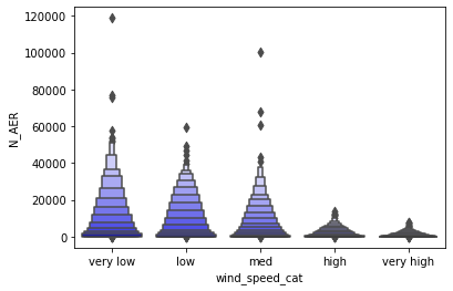
sns.displot(x="N_AER",hue = 'lat_cat',log_scale=True,kind='kde',
            data=df_ri,  multiple="stack")
<seaborn.axisgrid.FacetGrid at 0x7feac837ce20>
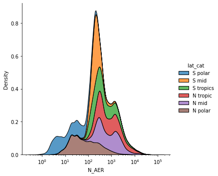
Convert back to xarray if we need:
ds_new = df_ri.set_index(['time','lat','lon']).to_xarray()
ds_new
<xarray.Dataset>
Dimensions:         (lat: 96, lon: 144, time: 36)
Coordinates:
  * time            (time) datetime64[ns] 2011-01-17 2011-02-14 ... 2013-12-17
  * lat             (lat) float64 -90.0 -88.11 -86.21 ... 86.21 88.11 90.0
  * lon             (lon) float64 -180.0 -177.5 -175.0 ... 172.5 175.0 177.5
Data variables: (12/13)
    lev             (time, lat, lon) float64 992.6 992.6 992.6 ... 992.6 992.6
    hyam            (time, lat, lon) float64 0.0 0.0 0.0 0.0 ... 0.0 0.0 0.0 0.0
    hybm            (time, lat, lon) float64 0.9926 0.9926 ... 0.9926 0.9926
    P0              (time, lat, lon) float64 1e+05 1e+05 1e+05 ... 1e+05 1e+05
    N_AER           (time, lat, lon) float32 29.52 29.52 29.52 ... 29.87 29.87
    PS              (time, lat, lon) float32 6.97e+04 6.97e+04 ... 1.012e+05
    ...              ...
    U               (time, lat, lon) float32 1.537 1.35 1.161 ... 3.829 3.874
    V               (time, lat, lon) float32 4.259 4.322 4.377 ... 1.122 0.9543
    T_C             (time, lat, lon) float32 -24.04 -24.04 ... -22.78 -22.78
    Wind_speed      (time, lat, lon) float32 4.528 4.528 4.528 ... 3.99 3.99
    wind_speed_cat  (time, lat, lon) object 'med' 'med' 'med' ... 'med' 'med'
lat_cat (time, lat, lon) object nan nan nan ... 'N polar' 'N polar'- lat: 96
- lon: 144
- time: 36
- time(time)datetime64[ns]2011-01-17 ... 2013-12-17
array(['2011-01-17T00:00:00.000000000', '2011-02-14T00:00:00.000000000', '2011-03-17T00:00:00.000000000', '2011-04-16T00:00:00.000000000', '2011-05-17T00:00:00.000000000', '2011-06-16T00:00:00.000000000', '2011-07-17T00:00:00.000000000', '2011-08-17T00:00:00.000000000', '2011-09-16T00:00:00.000000000', '2011-10-17T00:00:00.000000000', '2011-11-16T00:00:00.000000000', '2011-12-17T00:00:00.000000000', '2012-01-17T00:00:00.000000000', '2012-02-15T00:00:00.000000000', '2012-03-17T00:00:00.000000000', '2012-04-16T00:00:00.000000000', '2012-05-17T00:00:00.000000000', '2012-06-16T00:00:00.000000000', '2012-07-17T00:00:00.000000000', '2012-08-17T00:00:00.000000000', '2012-09-16T00:00:00.000000000', '2012-10-17T00:00:00.000000000', '2012-11-16T00:00:00.000000000', '2012-12-17T00:00:00.000000000', '2013-01-17T00:00:00.000000000', '2013-02-14T00:00:00.000000000', '2013-03-17T00:00:00.000000000', '2013-04-16T00:00:00.000000000', '2013-05-17T00:00:00.000000000', '2013-06-16T00:00:00.000000000', '2013-07-17T00:00:00.000000000', '2013-08-17T00:00:00.000000000', '2013-09-16T00:00:00.000000000', '2013-10-17T00:00:00.000000000', '2013-11-16T00:00:00.000000000', '2013-12-17T00:00:00.000000000'], dtype='datetime64[ns]') - lat(lat)float64-90.0 -88.11 -86.21 ... 88.11 90.0
array([-90. , -88.105263, -86.210526, -84.315789, -82.421053, -80.526316, -78.631579, -76.736842, -74.842105, -72.947368, -71.052632, -69.157895, -67.263158, -65.368421, -63.473684, -61.578947, -59.684211, -57.789474, -55.894737, -54. , -52.105263, -50.210526, -48.315789, -46.421053, -44.526316, -42.631579, -40.736842, -38.842105, -36.947368, -35.052632, -33.157895, -31.263158, -29.368421, -27.473684, -25.578947, -23.684211, -21.789474, -19.894737, -18. , -16.105263, -14.210526, -12.315789, -10.421053, -8.526316, -6.631579, -4.736842, -2.842105, -0.947368, 0.947368, 2.842105, 4.736842, 6.631579, 8.526316, 10.421053, 12.315789, 14.210526, 16.105263, 18. , 19.894737, 21.789474, 23.684211, 25.578947, 27.473684, 29.368421, 31.263158, 33.157895, 35.052632, 36.947368, 38.842105, 40.736842, 42.631579, 44.526316, 46.421053, 48.315789, 50.210526, 52.105263, 54. , 55.894737, 57.789474, 59.684211, 61.578947, 63.473684, 65.368421, 67.263158, 69.157895, 71.052632, 72.947368, 74.842105, 76.736842, 78.631579, 80.526316, 82.421053, 84.315789, 86.210526, 88.105263, 90. ]) - lon(lon)float64-180.0 -177.5 ... 175.0 177.5
array([-180. , -177.5, -175. , -172.5, -170. , -167.5, -165. , -162.5, -160. ,
       -157.5, -155. , -152.5, -150. , -147.5, -145. , -142.5, -140. , -137.5,
       -135. , -132.5, -130. , -127.5, -125. , -122.5, -120. , -117.5, -115. ,
       -112.5, -110. , -107.5, -105. , -102.5, -100. ,  -97.5,  -95. ,  -92.5,
        -90. ,  -87.5,  -85. ,  -82.5,  -80. ,  -77.5,  -75. ,  -72.5,  -70. ,
        -67.5,  -65. ,  -62.5,  -60. ,  -57.5,  -55. ,  -52.5,  -50. ,  -47.5,
        -45. ,  -42.5,  -40. ,  -37.5,  -35. ,  -32.5,  -30. ,  -27.5,  -25. ,
        -22.5,  -20. ,  -17.5,  -15. ,  -12.5,  -10. ,   -7.5,   -5. ,   -2.5,
          0. ,    2.5,    5. ,    7.5,   10. ,   12.5,   15. ,   17.5,   20. ,
         22.5,   25. ,   27.5,   30. ,   32.5,   35. ,   37.5,   40. ,   42.5,
         45. ,   47.5,   50. ,   52.5,   55. ,   57.5,   60. ,   62.5,   65. ,
         67.5,   70. ,   72.5,   75. ,   77.5,   80. ,   82.5,   85. ,   87.5,
         90. ,   92.5,   95. ,   97.5,  100. ,  102.5,  105. ,  107.5,  110. ,
        112.5,  115. ,  117.5,  120. ,  122.5,  125. ,  127.5,  130. ,  132.5,
        135. ,  137.5,  140. ,  142.5,  145. ,  147.5,  150. ,  152.5,  155. ,
        157.5,  160. ,  162.5,  165. ,  167.5,  170. ,  172.5,  175. ,  177.5])
- lev(time, lat, lon)float64992.6 992.6 992.6 ... 992.6 992.6
array([[[992.55609512, 992.55609512, 992.55609512, ..., 992.55609512, 992.55609512, 992.55609512], [992.55609512, 992.55609512, 992.55609512, ..., 992.55609512, 992.55609512, 992.55609512], [992.55609512, 992.55609512, 992.55609512, ..., 992.55609512, 992.55609512, 992.55609512], ..., [992.55609512, 992.55609512, 992.55609512, ..., 992.55609512, 992.55609512, 992.55609512], [992.55609512, 992.55609512, 992.55609512, ..., 992.55609512, 992.55609512, 992.55609512], [992.55609512, 992.55609512, 992.55609512, ..., 992.55609512, 992.55609512, 992.55609512]], [[992.55609512, 992.55609512, 992.55609512, ..., 992.55609512, 992.55609512, 992.55609512], [992.55609512, 992.55609512, 992.55609512, ..., 992.55609512, 992.55609512, 992.55609512], [992.55609512, 992.55609512, 992.55609512, ..., 992.55609512, 992.55609512, 992.55609512], ... [992.55609512, 992.55609512, 992.55609512, ..., 992.55609512, 992.55609512, 992.55609512], [992.55609512, 992.55609512, 992.55609512, ..., 992.55609512, 992.55609512, 992.55609512], [992.55609512, 992.55609512, 992.55609512, ..., 992.55609512, 992.55609512, 992.55609512]], [[992.55609512, 992.55609512, 992.55609512, ..., 992.55609512, 992.55609512, 992.55609512], [992.55609512, 992.55609512, 992.55609512, ..., 992.55609512, 992.55609512, 992.55609512], [992.55609512, 992.55609512, 992.55609512, ..., 992.55609512, 992.55609512, 992.55609512], ..., [992.55609512, 992.55609512, 992.55609512, ..., 992.55609512, 992.55609512, 992.55609512], [992.55609512, 992.55609512, 992.55609512, ..., 992.55609512, 992.55609512, 992.55609512], [992.55609512, 992.55609512, 992.55609512, ..., 992.55609512, 992.55609512, 992.55609512]]]) - hyam(time, lat, lon)float640.0 0.0 0.0 0.0 ... 0.0 0.0 0.0 0.0
array([[[0., 0., 0., ..., 0., 0., 0.], [0., 0., 0., ..., 0., 0., 0.], [0., 0., 0., ..., 0., 0., 0.], ..., [0., 0., 0., ..., 0., 0., 0.], [0., 0., 0., ..., 0., 0., 0.], [0., 0., 0., ..., 0., 0., 0.]], [[0., 0., 0., ..., 0., 0., 0.], [0., 0., 0., ..., 0., 0., 0.], [0., 0., 0., ..., 0., 0., 0.], ..., [0., 0., 0., ..., 0., 0., 0.], [0., 0., 0., ..., 0., 0., 0.], [0., 0., 0., ..., 0., 0., 0.]], [[0., 0., 0., ..., 0., 0., 0.], [0., 0., 0., ..., 0., 0., 0.], [0., 0., 0., ..., 0., 0., 0.], ..., ... ..., [0., 0., 0., ..., 0., 0., 0.], [0., 0., 0., ..., 0., 0., 0.], [0., 0., 0., ..., 0., 0., 0.]], [[0., 0., 0., ..., 0., 0., 0.], [0., 0., 0., ..., 0., 0., 0.], [0., 0., 0., ..., 0., 0., 0.], ..., [0., 0., 0., ..., 0., 0., 0.], [0., 0., 0., ..., 0., 0., 0.], [0., 0., 0., ..., 0., 0., 0.]], [[0., 0., 0., ..., 0., 0., 0.], [0., 0., 0., ..., 0., 0., 0.], [0., 0., 0., ..., 0., 0., 0.], ..., [0., 0., 0., ..., 0., 0., 0.], [0., 0., 0., ..., 0., 0., 0.], [0., 0., 0., ..., 0., 0., 0.]]]) - hybm(time, lat, lon)float640.9926 0.9926 ... 0.9926 0.9926
array([[[0.9925561, 0.9925561, 0.9925561, ..., 0.9925561, 0.9925561, 0.9925561], [0.9925561, 0.9925561, 0.9925561, ..., 0.9925561, 0.9925561, 0.9925561], [0.9925561, 0.9925561, 0.9925561, ..., 0.9925561, 0.9925561, 0.9925561], ..., [0.9925561, 0.9925561, 0.9925561, ..., 0.9925561, 0.9925561, 0.9925561], [0.9925561, 0.9925561, 0.9925561, ..., 0.9925561, 0.9925561, 0.9925561], [0.9925561, 0.9925561, 0.9925561, ..., 0.9925561, 0.9925561, 0.9925561]], [[0.9925561, 0.9925561, 0.9925561, ..., 0.9925561, 0.9925561, 0.9925561], [0.9925561, 0.9925561, 0.9925561, ..., 0.9925561, 0.9925561, 0.9925561], [0.9925561, 0.9925561, 0.9925561, ..., 0.9925561, 0.9925561, 0.9925561], ... [0.9925561, 0.9925561, 0.9925561, ..., 0.9925561, 0.9925561, 0.9925561], [0.9925561, 0.9925561, 0.9925561, ..., 0.9925561, 0.9925561, 0.9925561], [0.9925561, 0.9925561, 0.9925561, ..., 0.9925561, 0.9925561, 0.9925561]], [[0.9925561, 0.9925561, 0.9925561, ..., 0.9925561, 0.9925561, 0.9925561], [0.9925561, 0.9925561, 0.9925561, ..., 0.9925561, 0.9925561, 0.9925561], [0.9925561, 0.9925561, 0.9925561, ..., 0.9925561, 0.9925561, 0.9925561], ..., [0.9925561, 0.9925561, 0.9925561, ..., 0.9925561, 0.9925561, 0.9925561], [0.9925561, 0.9925561, 0.9925561, ..., 0.9925561, 0.9925561, 0.9925561], [0.9925561, 0.9925561, 0.9925561, ..., 0.9925561, 0.9925561, 0.9925561]]]) - P0(time, lat, lon)float641e+05 1e+05 1e+05 ... 1e+05 1e+05
array([[[100000., 100000., 100000., ..., 100000., 100000., 100000.], [100000., 100000., 100000., ..., 100000., 100000., 100000.], [100000., 100000., 100000., ..., 100000., 100000., 100000.], ..., [100000., 100000., 100000., ..., 100000., 100000., 100000.], [100000., 100000., 100000., ..., 100000., 100000., 100000.], [100000., 100000., 100000., ..., 100000., 100000., 100000.]], [[100000., 100000., 100000., ..., 100000., 100000., 100000.], [100000., 100000., 100000., ..., 100000., 100000., 100000.], [100000., 100000., 100000., ..., 100000., 100000., 100000.], ..., [100000., 100000., 100000., ..., 100000., 100000., 100000.], [100000., 100000., 100000., ..., 100000., 100000., 100000.], [100000., 100000., 100000., ..., 100000., 100000., 100000.]], [[100000., 100000., 100000., ..., 100000., 100000., 100000.], [100000., 100000., 100000., ..., 100000., 100000., 100000.], [100000., 100000., 100000., ..., 100000., 100000., 100000.], ..., ... ..., [100000., 100000., 100000., ..., 100000., 100000., 100000.], [100000., 100000., 100000., ..., 100000., 100000., 100000.], [100000., 100000., 100000., ..., 100000., 100000., 100000.]], [[100000., 100000., 100000., ..., 100000., 100000., 100000.], [100000., 100000., 100000., ..., 100000., 100000., 100000.], [100000., 100000., 100000., ..., 100000., 100000., 100000.], ..., [100000., 100000., 100000., ..., 100000., 100000., 100000.], [100000., 100000., 100000., ..., 100000., 100000., 100000.], [100000., 100000., 100000., ..., 100000., 100000., 100000.]], [[100000., 100000., 100000., ..., 100000., 100000., 100000.], [100000., 100000., 100000., ..., 100000., 100000., 100000.], [100000., 100000., 100000., ..., 100000., 100000., 100000.], ..., [100000., 100000., 100000., ..., 100000., 100000., 100000.], [100000., 100000., 100000., ..., 100000., 100000., 100000.], [100000., 100000., 100000., ..., 100000., 100000., 100000.]]]) - N_AER(time, lat, lon)float3229.52 29.52 29.52 ... 29.87 29.87
array([[[29.523746 , 29.523243 , 29.523315 , ..., 29.523018 , 29.522842 , 29.523087 ], [30.62785 , 30.037271 , 30.105543 , ..., 31.354881 , 31.740213 , 31.421618 ], [27.920774 , 28.918839 , 29.699617 , ..., 26.752884 , 26.831234 , 27.22184 ], ..., [22.248058 , 21.908642 , 21.525434 , ..., 23.58223 , 23.251677 , 22.688652 ], [24.718075 , 24.695045 , 24.546497 , ..., 25.216768 , 25.078747 , 24.85078 ], [22.366716 , 22.35961 , 22.359612 , ..., 22.35962 , 22.35962 , 22.359608 ]], [[44.145832 , 44.14588 , 44.1463 , ..., 44.145035 , 44.145134 , 44.145435 ], [39.207695 , 39.747017 , 40.62748 , ..., 39.15167 , 38.685135 , 38.78143 ], [45.82052 , 47.16626 , 48.093723 , ..., 43.9546 , 44.26349 , 44.862583 ], ... [12.595164 , 12.467785 , 12.21201 , ..., 13.723299 , 13.2679615, 12.844725 ], [14.235027 , 14.122585 , 14.018166 , ..., 14.432014 , 14.395307 , 14.305435 ], [16.920443 , 16.917957 , 16.921741 , ..., 16.917677 , 16.921463 , 16.921017 ]], [[21.499374 , 21.499647 , 21.499374 , ..., 21.501133 , 21.500975 , 21.500177 ], [19.232729 , 19.11012 , 19.068794 , ..., 20.093475 , 19.812859 , 19.465431 ], [20.796038 , 21.02478 , 21.21718 , ..., 20.904696 , 20.898123 , 20.821136 ], ..., [21.452791 , 21.683409 , 21.669895 , ..., 21.777552 , 21.448221 , 21.231123 ], [24.332853 , 24.100332 , 24.05743 , ..., 24.69338 , 24.415026 , 24.45249 ], [29.872524 , 29.872066 , 29.909327 , ..., 29.871275 , 29.871218 , 29.871033 ]]], dtype=float32) - PS(time, lat, lon)float326.97e+04 6.97e+04 ... 1.012e+05
array([[[ 69700.375, 69700.375, 69700.375, ..., 69700.375, 69700.375, 69700.375], [ 66578.05 , 66661.62 , 66747.73 , ..., 66514.805, 66534.234, 66555.44 ], [ 69405.31 , 69736.445, 70129.01 , ..., 69633.16 , 69524.51 , 69450.28 ], ..., [101739.93 , 101728.65 , 101716.31 , ..., 101686.734, 101705.94 , 101724.14 ], [101610.805, 101612.25 , 101614.2 , ..., 101587.01 , 101594.84 , 101603.055], [101537.68 , 101537.68 , 101537.68 , ..., 101537.68 , 101537.68 , 101537.68 ]], [[ 69311.914, 69311.914, 69311.914, ..., 69311.914, 69311.914, 69311.914], [ 66071.516, 66155.52 , 66242.49 , ..., 66009.76 , 66028.58 , 66049.07 ], [ 68855.33 , 69189.56 , 69585.91 , ..., 69070.64 , 68965.625, 68895.32 ], ... [100346.02 , 100343.38 , 100340.305, ..., 100268.66 , 100296.59 , 100322.69 ], [100244.37 , 100250.64 , 100257.82 , ..., 100207.84 , 100219.87 , 100232.14 ], [100154.625, 100154.625, 100154.625, ..., 100154.625, 100154.625, 100154.625]], [[ 69259.05 , 69259.05 , 69259.05 , ..., 69259.05 , 69259.05 , 69259.05 ], [ 66109.74 , 66193.05 , 66279.27 , ..., 66048.05 , 66067.195, 66087.766], [ 68954.234, 69286.72 , 69680.055, ..., 69178.26 , 69071.72 , 68998.03 ], ..., [101704.84 , 101688.664, 101671.09 , ..., 101663.03 , 101679.836, 101693.9 ], [101438.78 , 101436.6 , 101434.734, ..., 101425.234, 101429.664, 101434.29 ], [101193.19 , 101193.19 , 101193.19 , ..., 101193.19 , 101193.19 , 101193.19 ]]], dtype=float32) - T(time, lat, lon)float32249.1 249.1 249.1 ... 250.4 250.4
array([[[249.11302, 249.1117 , 249.11102, ..., 249.11604, 249.1152 , 249.11427], [246.81152, 246.9152 , 247.03442, ..., 246.69734, 246.73514, 246.76639], [249.19638, 249.60878, 249.9665 , ..., 249.11742, 249.12567, 249.1915 ], ..., [242.55553, 242.43347, 242.35649, ..., 242.86372, 242.77458, 242.67116], [242.54964, 242.46341, 242.4001 , ..., 242.72894, 242.66245, 242.60161], [242.41449, 242.41441, 242.41441, ..., 242.41443, 242.41443, 242.4144 ]], [[239.8294 , 239.82794, 239.82701, ..., 239.83298, 239.8321 , 239.83095], [238.82741, 238.958 , 239.09895, ..., 238.62178, 238.68784, 238.75116], [243.58517, 244.10162, 244.49367, ..., 243.09366, 243.23161, 243.46527], ... [248.04962, 248.11653, 248.20952, ..., 247.97675, 247.97284, 248.0013 ], [248.14569, 248.1596 , 248.18814, ..., 248.15515, 248.14502, 248.14276], [247.8432 , 247.84323, 247.84325, ..., 247.84323, 247.84322, 247.8432 ]], [[247.59232, 247.59103, 247.59016, ..., 247.5954 , 247.59467, 247.59361], [245.81966, 245.90181, 246.00478, ..., 245.71089, 245.74902, 245.79836], [248.80498, 249.23846, 249.72571, ..., 248.62053, 248.6461 , 248.76117], ..., [247.10567, 246.98549, 246.87996, ..., 247.47267, 247.33858, 247.21783], [248.44025, 248.41652, 248.42267, ..., 248.53508, 248.49257, 248.4619 ], [250.37035, 250.37032, 250.37032, ..., 250.3703 , 250.37029, 250.3703 ]]], dtype=float32) - U(time, lat, lon)float321.537 1.35 1.161 ... 3.829 3.874
array([[[ 1.5370315 , 1.3503286 , 1.1607155 , ..., 2.0783696 , 1.901378 , 1.7208107 ], [-1.159901 , -1.2303753 , -1.2994658 , ..., -0.90470093, -0.99685 , -1.08114 ], [-0.32837594, -0.40894952, -0.48456272, ..., -0.30095586, -0.29538855, -0.30268258], ..., [ 1.3737727 , 1.3725647 , 1.3676085 , ..., 1.3562961 , 1.3657501 , 1.3701768 ], [ 0.9682078 , 0.9809572 , 0.99107885, ..., 0.9141902 , 0.9344501 , 0.9527456 ], [ 0.47931617, 0.48669425, 0.49314618, ..., 0.4517723 , 0.46183804, 0.47102764]], [[ 2.0534956 , 1.837702 , 1.6184766 , ..., 2.6757553 , 2.472942 , 2.2654014 ], [-2.4265878 , -2.4840286 , -2.5341287 , ..., -2.18238 , -2.2781904 , -2.36032 ], [-0.7626382 , -0.7645772 , -0.82423496, ..., -0.87721634, -0.80213517, -0.78119445], ... [ 0.99942106, 1.1151545 , 1.2295555 , ..., 0.6288369 , 0.7550915 , 0.8795819 ], [ 0.37215477, 0.4961984 , 0.6205809 , ..., -0.02273837, 0.11161902, 0.24428926], [-0.5593583 , -0.4418575 , -0.32347158, ..., -0.9047558 , -0.79106903, -0.6758832 ]], [[ 1.0580302 , 0.8989314 , 0.7378481 , ..., 1.5213714 , 1.3693111 , 1.2148681 ], [-1.5714442 , -1.6363475 , -1.6942055 , ..., -1.3093575 , -1.4073235 , -1.4966952 ], [-0.6840069 , -0.77011675, -0.9209507 , ..., -0.56274885, -0.5749575 , -0.6138484 ], ..., [ 4.835415 , 4.908922 , 4.964643 , ..., 4.486007 , 4.6191554 , 4.7365546 ], [ 4.6164155 , 4.674333 , 4.717868 , ..., 4.3664203 , 4.4622593 , 4.546965 ], [ 3.9122448 , 3.942795 , 3.965724 , ..., 3.7764134 , 3.8290284 , 3.8743227 ]]], dtype=float32) - V(time, lat, lon)float324.259 4.322 4.377 ... 1.122 0.9543
array([[[ 4.25897 , 4.3222117 , 4.377001 , ..., 4.021294 , 4.108306 , 4.187636 ], [ 4.772556 , 4.808405 , 4.830144 , ..., 4.629327 , 4.6838074 , 4.732354 ], [ 5.544316 , 5.4197598 , 5.2695813 , ..., 5.8627696 , 5.773715 , 5.6687565 ], ..., [ 0.36777872, 0.30199626, 0.23630716, ..., 0.55977666, 0.49940357, 0.4335238 ], [ 0.12903874, 0.05245972, -0.0201028 , ..., 0.36010763, 0.283067 , 0.20623507], [ 0.17959046, 0.15851356, 0.13713335, ..., 0.24061765, 0.22068258, 0.20032828]], [[ 4.899427 , 4.9843283 , 5.0596156 , ..., 4.589449 , 4.7017603 , 4.80517 ], [ 6.198694 , 6.2279706 , 6.247806 , ..., 6.085516 , 6.1295495 , 6.1683946 ], [ 7.9235854 , 7.835197 , 7.7261877 , ..., 8.074489 , 8.04273 , 7.9988203 ], ... [ 2.7846189 , 2.7389946 , 2.696448 , ..., 2.8643088 , 2.847608 , 2.820138 ], [ 2.5052292 , 2.4873688 , 2.4693673 , ..., 2.5303905 , 2.5258188 , 2.5171514 ], [ 2.6826248 , 2.7044697 , 2.7211623 , ..., 2.586665 , 2.6236908 , 2.6556602 ]], [[ 3.6324532 , 3.6760986 , 3.7122478 , ..., 3.4610398 , 3.5245912 , 3.581787 ], [ 3.675836 , 3.6573017 , 3.626574 , ..., 3.7165873 , 3.7068126 , 3.6905723 ], [ 5.0195146 , 4.9144697 , 4.8032837 , ..., 5.259472 , 5.194883 , 5.1188684 ], ..., [ 1.3250982 , 1.0564015 , 0.7830102 , ..., 2.0796602 , 1.8382746 , 1.5874441 ], [ 1.1074082 , 0.8779225 , 0.6460112 , ..., 1.7781768 , 1.557939 , 1.3348291 ], [ 0.7843159 , 0.61294866, 0.44039544, ..., 1.2882968 , 1.1223469 , 0.9542675 ]]], dtype=float32) - T_C(time, lat, lon)float32-24.04 -24.04 ... -22.78 -22.78
array([[[-24.036972 , -24.0383 , -24.03897 , ..., -24.03395 , -24.03479 , -24.03572 ], [-26.33847 , -26.234787 , -26.11557 , ..., -26.452652 , -26.414856 , -26.383606 ], [-23.953613 , -23.541214 , -23.183487 , ..., -24.032578 , -24.024323 , -23.958496 ], ..., [-30.594467 , -30.716522 , -30.793503 , ..., -30.28627 , -30.375412 , -30.478836 ], [-30.600357 , -30.686584 , -30.749893 , ..., -30.421051 , -30.487549 , -30.548386 ], [-30.735504 , -30.73558 , -30.73558 , ..., -30.735565 , -30.735565 , -30.735596 ]], [[-33.320587 , -33.322052 , -33.322983 , ..., -33.317017 , -33.317886 , -33.319046 ], [-34.322586 , -34.192 , -34.05104 , ..., -34.528214 , -34.46216 , -34.398834 ], [-29.56482 , -29.04837 , -28.656326 , ..., -30.056335 , -29.91838 , -29.684723 ], ... [-25.100372 , -25.033463 , -24.940475 , ..., -25.173248 , -25.177155 , -25.148697 ], [-25.004303 , -24.990387 , -24.961853 , ..., -24.994843 , -25.004974 , -25.007233 ], [-25.306793 , -25.306763 , -25.306747 , ..., -25.306763 , -25.306778 , -25.306793 ]], [[-25.557678 , -25.55896 , -25.55983 , ..., -25.554596 , -25.555328 , -25.556381 ], [-27.330338 , -27.248184 , -27.145218 , ..., -27.439102 , -27.40097 , -27.351639 ], [-24.345016 , -23.91153 , -23.424286 , ..., -24.529465 , -24.503891 , -24.388824 ], ..., [-26.044327 , -26.164505 , -26.270035 , ..., -25.677322 , -25.811417 , -25.93216 ], [-24.709747 , -24.733475 , -24.727325 , ..., -24.614914 , -24.657425 , -24.688095 ], [-22.779648 , -22.779678 , -22.779678 , ..., -22.779694 , -22.779709 , -22.779694 ]]], dtype=float32) - Wind_speed(time, lat, lon)float324.528 4.528 4.528 ... 3.99 3.99
array([[[ 4.527835 , 4.528234 , 4.5282884 , ..., 4.526635 , 4.5269656 , 4.527415 ], [ 4.9114823 , 4.9633236 , 5.0018897 , ..., 4.7169003 , 4.788712 , 4.8542805 ], [ 5.554032 , 5.435167 , 5.2918134 , ..., 5.870489 , 5.781266 , 5.6768317 ], ..., [ 1.4221507 , 1.4053952 , 1.387874 , ..., 1.4672726 , 1.454193 , 1.4371247 ], [ 0.9767688 , 0.98235893, 0.9912827 , ..., 0.9825585 , 0.9763831 , 0.9748113 ], [ 0.5118562 , 0.5118573 , 0.5118581 , ..., 0.5118545 , 0.51185465, 0.5118578 ]], [[ 5.3123655 , 5.312314 , 5.3121724 , ..., 5.312505 , 5.3124375 , 5.3124104 ], [ 6.6567364 , 6.705074 , 6.7421722 , ..., 6.465005 , 6.53923 , 6.604559 ], [ 7.960202 , 7.872413 , 7.7700286 , ..., 8.122 , 8.082631 , 8.036877 ], ... [ 2.9585376 , 2.9573064 , 2.9635518 , ..., 2.9325247 , 2.9460201 , 2.954123 ], [ 2.5327203 , 2.5363786 , 2.546153 , ..., 2.5304925 , 2.5282838 , 2.5289776 ], [ 2.7403207 , 2.7403274 , 2.740321 , ..., 2.740332 , 2.7403548 , 2.740319 ]], [[ 3.7834039 , 3.7844126 , 3.7848651 , ..., 3.780657 , 3.7812374 , 3.7822087 ], [ 3.9976504 , 4.0066805 , 4.002795 , ..., 3.9404871 , 3.964974 , 3.9825141 ], [ 5.0659046 , 4.974444 , 4.8907757 , ..., 5.2894926 , 5.2266035 , 5.155543 ], ..., [ 5.0136933 , 5.0213046 , 5.026011 , ..., 4.9446177 , 4.9715037 , 4.995491 ], [ 4.747383 , 4.7560635 , 4.7618914 , ..., 4.714609 , 4.726408 , 4.738846 ], [ 3.9900892 , 3.9901552 , 3.990102 , ..., 3.9901137 , 3.9901278 , 3.990113 ]]], dtype=float32) - wind_speed_cat(time, lat, lon)object'med' 'med' 'med' ... 'med' 'med'
array([[['med', 'med', 'med', ..., 'med', 'med', 'med'], ['med', 'med', 'med', ..., 'med', 'med', 'med'], ['high', 'med', 'med', ..., 'high', 'high', 'high'], ..., ['very low', 'very low', 'very low', ..., 'very low', 'very low', 'very low'], ['very low', 'very low', 'very low', ..., 'very low', 'very low', 'very low'], [nan, nan, nan, ..., nan, nan, nan]], [['med', 'med', 'med', ..., 'med', 'med', 'med'], ['high', 'high', 'high', ..., 'high', 'high', 'high'], ['very high', 'very high', 'very high', ..., 'very high', 'very high', 'very high'], ..., ['med', 'med', 'med', ..., 'med', 'med', 'med'], ['med', 'med', 'med', ..., 'med', 'med', 'med'], ['low', 'low', 'low', ..., 'low', 'low', 'low']], [['high', 'high', 'high', ..., 'high', 'high', 'high'], ... ['med', 'med', 'med', ..., 'med', 'med', 'med'], ['med', 'med', 'med', ..., 'med', 'med', 'med']], [['high', 'high', 'high', ..., 'high', 'high', 'high'], ['very high', 'very high', 'very high', ..., 'very high', 'very high', 'very high'], ['very high', 'very high', 'very high', ..., nan, 'very high', 'very high'], ..., ['med', 'med', 'med', ..., 'med', 'med', 'med'], ['low', 'low', 'low', ..., 'low', 'low', 'low'], ['med', 'med', 'med', ..., 'med', 'med', 'med']], [['med', 'med', 'med', ..., 'med', 'med', 'med'], ['med', 'med', 'med', ..., 'med', 'med', 'med'], ['med', 'med', 'med', ..., 'med', 'med', 'med'], ..., ['med', 'med', 'med', ..., 'med', 'med', 'med'], ['med', 'med', 'med', ..., 'med', 'med', 'med'], ['med', 'med', 'med', ..., 'med', 'med', 'med']]], dtype=object) - lat_cat(time, lat, lon)objectnan nan nan ... 'N polar' 'N polar'
array([[[nan, nan, nan, ..., nan, nan, nan],
        ['S polar', 'S polar', 'S polar', ..., 'S polar', 'S polar',
         'S polar'],
        ['S polar', 'S polar', 'S polar', ..., 'S polar', 'S polar',
         'S polar'],
        ...,
        ['N polar', 'N polar', 'N polar', ..., 'N polar', 'N polar',
         'N polar'],
        ['N polar', 'N polar', 'N polar', ..., 'N polar', 'N polar',
         'N polar'],
        ['N polar', 'N polar', 'N polar', ..., 'N polar', 'N polar',
         'N polar']],

       [[nan, nan, nan, ..., nan, nan, nan],
        ['S polar', 'S polar', 'S polar', ..., 'S polar', 'S polar',
         'S polar'],
        ['S polar', 'S polar', 'S polar', ..., 'S polar', 'S polar',
         'S polar'],
        ...,
        ['N polar', 'N polar', 'N polar', ..., 'N polar', 'N polar',
...
        ...,
        ['N polar', 'N polar', 'N polar', ..., 'N polar', 'N polar',
         'N polar'],
        ['N polar', 'N polar', 'N polar', ..., 'N polar', 'N polar',
         'N polar'],
        ['N polar', 'N polar', 'N polar', ..., 'N polar', 'N polar',
         'N polar']],

       [[nan, nan, nan, ..., nan, nan, nan],
        ['S polar', 'S polar', 'S polar', ..., 'S polar', 'S polar',
         'S polar'],
        ['S polar', 'S polar', 'S polar', ..., 'S polar', 'S polar',
         'S polar'],
        ...,
        ['N polar', 'N polar', 'N polar', ..., 'N polar', 'N polar',
         'N polar'],
        ['N polar', 'N polar', 'N polar', ..., 'N polar', 'N polar',
         'N polar'],
        ['N polar', 'N polar', 'N polar', ..., 'N polar', 'N polar',
         'N polar']]], dtype=object)
Groupby
ds_new.where(ds_new['wind_speed_cat']=='low').mean('time')['N_AER'].plot()
<matplotlib.collections.QuadMesh at 0x7feac80d2b80>
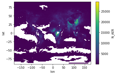
ds['wind_speed'] = np.sqrt(ds['U']**2+ ds['V']**2)
ds_new.groupby('wind_speed_cat').mean()
<xarray.Dataset>
Dimensions:         (wind_speed_cat: 5)
Coordinates:
  * wind_speed_cat  (wind_speed_cat) object 'high' 'low' ... 'very low'
Data variables:
    lev             (wind_speed_cat) float64 992.6 992.6 992.6 992.6 992.6
    hyam            (wind_speed_cat) float64 0.0 0.0 0.0 0.0 0.0
    hybm            (wind_speed_cat) float64 0.9926 0.9926 0.9926 0.9926 0.9926
    P0              (wind_speed_cat) float64 1e+05 1e+05 1e+05 1e+05 1e+05
    N_AER           (wind_speed_cat) float32 329.0 1.117e+03 ... 237.5 1.437e+03
    PS              (wind_speed_cat) float32 9.642e+04 9.782e+04 ... 9.712e+04
    T               (wind_speed_cat) float32 279.2 279.3 279.2 273.2 280.1
    U               (wind_speed_cat) float32 -0.7335 0.06986 ... -0.1049 0.02193
    V               (wind_speed_cat) float32 0.4115 0.04852 ... 0.3027 -0.01771
    T_C             (wind_speed_cat) float32 6.061 6.121 6.028 0.01729 6.922
Wind_speed (wind_speed_cat) float32 6.476 2.127 3.922 8.538 1.218- wind_speed_cat: 5
- wind_speed_cat(wind_speed_cat)object'high' 'low' ... 'very low'
array(['high', 'low', 'med', 'very high', 'very low'], dtype=object)
- lev(wind_speed_cat)float64992.6 992.6 992.6 992.6 992.6
array([992.55609512, 992.55609512, 992.55609512, 992.55609512, 992.55609512]) - hyam(wind_speed_cat)float640.0 0.0 0.0 0.0 0.0
array([0., 0., 0., 0., 0.])
- hybm(wind_speed_cat)float640.9926 0.9926 0.9926 0.9926 0.9926
array([0.9925561, 0.9925561, 0.9925561, 0.9925561, 0.9925561])
- P0(wind_speed_cat)float641e+05 1e+05 1e+05 1e+05 1e+05
array([100000., 100000., 100000., 100000., 100000.])
- N_AER(wind_speed_cat)float32329.0 1.117e+03 ... 237.5 1.437e+03
array([ 329.0471 , 1117.213 , 628.59357, 237.45853, 1436.5134 ], dtype=float32) - PS(wind_speed_cat)float329.642e+04 9.782e+04 ... 9.712e+04
array([96415.945, 97816.125, 97850.65 , 94217.12 , 97115.64 ], dtype=float32) - T(wind_speed_cat)float32279.2 279.3 279.2 273.2 280.1
array([279.21072, 279.27063, 279.1781 , 273.1673 , 280.07236], dtype=float32) - U(wind_speed_cat)float32-0.7335 0.06986 ... -0.1049 0.02193
array([-0.73346454, 0.06986377, -0.01202026, -0.10492255, 0.02193465], dtype=float32) - V(wind_speed_cat)float320.4115 0.04852 ... 0.3027 -0.01771
array([ 0.4115437 , 0.04852395, 0.23771387, 0.3026635 , -0.01771242], dtype=float32) - T_C(wind_speed_cat)float326.061 6.121 6.028 0.01729 6.922
array([6.0607424 , 6.1206164 , 6.0281363 , 0.01729127, 6.9223757 ], dtype=float32) - Wind_speed(wind_speed_cat)float326.476 2.127 3.922 8.538 1.218
array([6.475609 , 2.126911 , 3.9222631, 8.538465 , 1.2179215],
      dtype=float32)
df[['U','V']].plot.hist(alpha=0.5, bins=200)
<AxesSubplot:ylabel='Frequency'>

df_tjarno.head()
| lat | lon | lev | hyam | hybm | P0 | N_AER | PS | T | U | V | T_C | |
|---|---|---|---|---|---|---|---|---|---|---|---|---|
| time | ||||||||||||
| 2011-01-17 | 59.684211 | 10.0 | 992.556095 | 0.0 | 0.992556 | 100000.0 | 708.058899 | 96880.921875 | 269.207245 | 1.728664 | 0.475478 | -3.942749 |
| 2011-02-14 | 59.684211 | 10.0 | 992.556095 | 0.0 | 0.992556 | 100000.0 | 830.089844 | 97367.218750 | 266.607880 | -0.424161 | 1.017061 | -6.542114 |
| 2011-03-17 | 59.684211 | 10.0 | 992.556095 | 0.0 | 0.992556 | 100000.0 | 585.032104 | 97448.093750 | 271.787231 | 2.352789 | 0.320621 | -1.362762 |
| 2011-04-16 | 59.684211 | 10.0 | 992.556095 | 0.0 | 0.992556 | 100000.0 | 906.228210 | 97496.757812 | 279.498474 | 1.632975 | -0.223941 | 6.348480 |
| 2011-05-17 | 59.684211 | 10.0 | 992.556095 | 0.0 | 0.992556 | 100000.0 | 872.936096 | 97293.382812 | 281.770081 | 1.449824 | 1.465539 | 8.620087 |