From xarray to pandas
Contents
From xarray to pandas
Import python packages
import xarray as xr
xr.set_options(display_style='html')
import intake
import cftime
import matplotlib.pyplot as plt
import cartopy.crs as ccrs
import pandas as pd
import dask
%matplotlib inline
Open CMIP6 online catalog
cat_url = "https://storage.googleapis.com/cmip6/pangeo-cmip6.json"
col = intake.open_esm_datastore(cat_url)
col
pangeo-cmip6 catalog with 7632 dataset(s) from 517667 asset(s):
| unique | |
|---|---|
| activity_id | 18 |
| institution_id | 36 |
| source_id | 88 |
| experiment_id | 170 |
| member_id | 657 |
| table_id | 37 |
| variable_id | 709 |
| grid_label | 10 |
| zstore | 517667 |
| dcpp_init_year | 60 |
| version | 715 |
Search corresponding data
cat = col.search(source_id=['CESM2-WACCM'], experiment_id=['historical'], table_id=['AERmon'], variable_id=['so2'], member_id=['r1i1p1f1'])
cat.df
| activity_id | institution_id | source_id | experiment_id | member_id | table_id | variable_id | grid_label | zstore | dcpp_init_year | version | |
|---|---|---|---|---|---|---|---|---|---|---|---|
| 0 | CMIP | NCAR | CESM2-WACCM | historical | r1i1p1f1 | AERmon | so2 | gn | gs://cmip6/CMIP6/CMIP/NCAR/CESM2-WACCM/histori... | NaN | 20190227 |
Create dictionary from the list of datasets we found
This step may take several minutes so be patient!
dset_dict = cat.to_dataset_dict(zarr_kwargs={'use_cftime':True})
--> The keys in the returned dictionary of datasets are constructed as follows:
	'activity_id.institution_id.source_id.experiment_id.table_id.grid_label'
100.00% [1/1 00:00<00:00]
lconf = list(dset_dict.keys())
print(lconf)
['CMIP.NCAR.CESM2-WACCM.historical.AERmon.gn']
Open dataset
Use
xarraypython package to analyze netCDF datasetopen_datasetallows to get all the metadata without loading data into memory.with
xarray, we only load into memory what is needed.
dset = dset_dict[lconf[0]]
dset = dset.squeeze()
Get metadata corresponding to the whole dataset
dset
<xarray.Dataset>
Dimensions:    (lat: 192, lev: 70, lon: 288, nbnd: 2, time: 1980)
Coordinates:
  * lat        (lat) float64 -90.0 -89.06 -88.12 -87.17 ... 88.12 89.06 90.0
    lat_bnds   (lat, nbnd) float32 dask.array<chunksize=(192, 2), meta=np.ndarray>
  * lev        (lev) float64 -5.96e-06 -9.827e-06 -1.62e-05 ... -976.3 -992.6
    lev_bnds   (lev, nbnd) float32 dask.array<chunksize=(70, 2), meta=np.ndarray>
  * lon        (lon) float64 0.0 1.25 2.5 3.75 5.0 ... 355.0 356.2 357.5 358.8
    lon_bnds   (lon, nbnd) float32 dask.array<chunksize=(288, 2), meta=np.ndarray>
  * time       (time) object 1850-01-15 12:00:00 ... 2014-12-15 12:00:00
    time_bnds  (time, nbnd) object dask.array<chunksize=(1980, 2), meta=np.ndarray>
    member_id  <U8 'r1i1p1f1'
Dimensions without coordinates: nbnd
Data variables:
    so2        (time, lev, lat, lon) float32 dask.array<chunksize=(5, 70, 192, 288), meta=np.ndarray>
Attributes: (12/48)
    Conventions:             CF-1.7 CMIP-6.2
    activity_id:             CMIP
    branch_method:           standard
    branch_time_in_child:    674885.0
    branch_time_in_parent:   20075.0
    case_id:                 4
    ...                      ...
    variable_id:             so2
    variant_info:            CMIP6 CESM2 hindcast (1850-2014) with high-top a...
    variant_label:           r1i1p1f1
    status:                  2019-11-05;created;by nhn2@columbia.edu
    intake_esm_varname:      ['so2']
    intake_esm_dataset_key:  CMIP.NCAR.CESM2-WACCM.historical.AERmon.gn
xarray.Dataset
- lat: 192
- lev: 70
- lon: 288
- nbnd: 2
- time: 1980
- lat(lat)float64-90.0 -89.06 -88.12 ... 89.06 90.0
- axis :
- Y
- bounds :
- lat_bnds
- standard_name :
- latitude
- title :
- Latitude
- type :
- double
- units :
- degrees_north
- valid_max :
- 90.0
- valid_min :
- -90.0
array([-90. , -89.057592, -88.115183, -87.172775, -86.230366, -85.287958, -84.34555 , -83.403141, -82.460733, -81.518325, -80.575916, -79.633508, -78.691099, -77.748691, -76.806283, -75.863874, -74.921466, -73.979058, -73.036649, -72.094241, -71.151832, -70.209424, -69.267016, -68.324607, -67.382199, -66.439791, -65.497382, -64.554974, -63.612565, -62.670157, -61.727749, -60.78534 , -59.842932, -58.900524, -57.958115, -57.015707, -56.073298, -55.13089 , -54.188482, -53.246073, -52.303665, -51.361257, -50.418848, -49.47644 , -48.534031, -47.591623, -46.649215, -45.706806, -44.764398, -43.82199 , -42.879581, -41.937173, -40.994764, -40.052356, -39.109948, -38.167539, -37.225131, -36.282723, -35.340314, -34.397906, -33.455497, -32.513089, -31.570681, -30.628272, -29.685864, -28.743455, -27.801047, -26.858639, -25.91623 , -24.973822, -24.031414, -23.089005, -22.146597, -21.204188, -20.26178 , -19.319372, -18.376963, -17.434555, -16.492147, -15.549738, -14.60733 , -13.664921, -12.722513, -11.780105, -10.837696, -9.895288, -8.95288 , -8.010471, -7.068063, -6.125654, -5.183246, -4.240838, -3.298429, -2.356021, -1.413613, -0.471204, 0.471204, 1.413613, 2.356021, 3.298429, 4.240838, 5.183246, 6.125654, 7.068063, 8.010471, 8.95288 , 9.895288, 10.837696, 11.780105, 12.722513, 13.664921, 14.60733 , 15.549738, 16.492147, 17.434555, 18.376963, 19.319372, 20.26178 , 21.204188, 22.146597, 23.089005, 24.031414, 24.973822, 25.91623 , 26.858639, 27.801047, 28.743455, 29.685864, 30.628272, 31.570681, 32.513089, 33.455497, 34.397906, 35.340314, 36.282723, 37.225131, 38.167539, 39.109948, 40.052356, 40.994764, 41.937173, 42.879581, 43.82199 , 44.764398, 45.706806, 46.649215, 47.591623, 48.534031, 49.47644 , 50.418848, 51.361257, 52.303665, 53.246073, 54.188482, 55.13089 , 56.073298, 57.015707, 57.958115, 58.900524, 59.842932, 60.78534 , 61.727749, 62.670157, 63.612565, 64.554974, 65.497382, 66.439791, 67.382199, 68.324607, 69.267016, 70.209424, 71.151832, 72.094241, 73.036649, 73.979058, 74.921466, 75.863874, 76.806283, 77.748691, 78.691099, 79.633508, 80.575916, 81.518325, 82.460733, 83.403141, 84.34555 , 85.287958, 86.230366, 87.172775, 88.115183, 89.057592, 90. ]) - lat_bnds(lat, nbnd)float32dask.array<chunksize=(192, 2), meta=np.ndarray>
- units :
- degrees_north
Array Chunk Bytes 1.54 kB 1.54 kB Shape (192, 2) (192, 2) Count 2 Tasks 1 Chunks Type float32 numpy.ndarray - lev(lev)float64-5.96e-06 -9.827e-06 ... -992.6
- axis :
- Z
- bounds :
- lev_bnds
- positive :
- up
- standard_name :
- alevel
- title :
- atmospheric model level
- type :
- double
- units :
- hPa
array([-5.960300e-06, -9.826900e-06, -1.620185e-05, -2.671225e-05, -4.404100e-05, -7.261275e-05, -1.197190e-04, -1.973800e-04, -3.254225e-04, -5.365325e-04, -8.846025e-04, -1.458457e-03, -2.404575e-03, -3.978250e-03, -6.556826e-03, -1.081383e-02, -1.789800e-02, -2.955775e-02, -4.873075e-02, -7.991075e-02, -1.282732e-01, -1.981200e-01, -2.920250e-01, -4.101675e-01, -5.534700e-01, -7.304800e-01, -9.559475e-01, -1.244795e+00, -1.612850e+00, -2.079325e+00, -2.667425e+00, -3.404875e+00, -4.324575e+00, -5.465400e+00, -6.872850e+00, -8.599725e+00, -1.070705e+01, -1.326475e+01, -1.635175e+01, -2.005675e+01, -2.447900e+01, -2.972800e+01, -3.592325e+01, -4.319375e+01, -5.167750e+01, -6.152050e+01, -7.375096e+01, -8.782123e+01, -1.033171e+02, -1.215472e+02, -1.429940e+02, -1.682251e+02, -1.979081e+02, -2.328286e+02, -2.739108e+02, -3.222419e+02, -3.791009e+02, -4.459926e+02, -5.246872e+02, -6.097787e+02, -6.913894e+02, -7.634045e+02, -8.208584e+02, -8.595348e+02, -8.870202e+02, -9.126445e+02, -9.361984e+02, -9.574855e+02, -9.763254e+02, -9.925561e+02]) - lev_bnds(lev, nbnd)float32dask.array<chunksize=(70, 2), meta=np.ndarray>
- formula :
- p = a*p0 + b*ps
- formula_terms :
- p0: p0 a: a_bnds b: b_bnds ps: ps
- standard_name :
- atmosphere_hybrid_sigma_pressure_coordinate
- units :
- hPa
Array Chunk Bytes 560 B 560 B Shape (70, 2) (70, 2) Count 2 Tasks 1 Chunks Type float32 numpy.ndarray - lon(lon)float640.0 1.25 2.5 ... 356.2 357.5 358.8
- axis :
- X
- bounds :
- lon_bnds
- standard_name :
- longitude
- title :
- Longitude
- type :
- double
- units :
- degrees_east
- valid_max :
- 360.0
- valid_min :
- 0.0
array([ 0. , 1.25, 2.5 , ..., 356.25, 357.5 , 358.75])
- lon_bnds(lon, nbnd)float32dask.array<chunksize=(288, 2), meta=np.ndarray>
- units :
- degrees_east
Array Chunk Bytes 2.30 kB 2.30 kB Shape (288, 2) (288, 2) Count 2 Tasks 1 Chunks Type float32 numpy.ndarray - time(time)object1850-01-15 12:00:00 ... 2014-12-...
- axis :
- T
- bounds :
- time_bnds
- standard_name :
- time
- title :
- time
- type :
- double
array([cftime.DatetimeNoLeap(1850, 1, 15, 12, 0, 0, 0), cftime.DatetimeNoLeap(1850, 2, 14, 0, 0, 0, 0), cftime.DatetimeNoLeap(1850, 3, 15, 12, 0, 0, 0), ..., cftime.DatetimeNoLeap(2014, 10, 15, 12, 0, 0, 0), cftime.DatetimeNoLeap(2014, 11, 15, 0, 0, 0, 0), cftime.DatetimeNoLeap(2014, 12, 15, 12, 0, 0, 0)], dtype=object) - time_bnds(time, nbnd)objectdask.array<chunksize=(1980, 2), meta=np.ndarray>
Array Chunk Bytes 31.68 kB 31.68 kB Shape (1980, 2) (1980, 2) Count 2 Tasks 1 Chunks Type object numpy.ndarray - member_id()<U8'r1i1p1f1'
array('r1i1p1f1', dtype='<U8')
- so2(time, lev, lat, lon)float32dask.array<chunksize=(5, 70, 192, 288), meta=np.ndarray>
- cell_measures :
- area: areacella
- cell_methods :
- area: time: mean
- comment :
- Mole fraction is used in the construction mole_fraction_of_X_in_Y, where X is a material constituent of Y.
- description :
- Mole fraction is used in the construction mole_fraction_of_X_in_Y, where X is a material constituent of Y.
- frequency :
- mon
- id :
- so2
- long_name :
- SO2 Volume Mixing Ratio
- mipTable :
- AERmon
- out_name :
- so2
- prov :
- AERmon ((isd.003))
- realm :
- aerosol
- standard_name :
- mole_fraction_of_sulfur_dioxide_in_air
- time :
- time
- time_label :
- time-mean
- time_title :
- Temporal mean
- title :
- SO2 Volume Mixing Ratio
- type :
- real
- units :
- mol mol-1
- variable_id :
- so2
Array Chunk Bytes 30.66 GB 77.41 MB Shape (1980, 70, 192, 288) (5, 70, 192, 288) Count 1189 Tasks 396 Chunks Type float32 numpy.ndarray
- Conventions :
- CF-1.7 CMIP-6.2
- activity_id :
- CMIP
- branch_method :
- standard
- branch_time_in_child :
- 674885.0
- branch_time_in_parent :
- 20075.0
- case_id :
- 4
- cesm_casename :
- b.e21.BWHIST.f09_g17.CMIP6-historical-WACCM.001
- contact :
- cesm_cmip6@ucar.edu
- creation_date :
- 2019-01-31T00:49:45Z
- data_specs_version :
- 01.00.29
- experiment :
- all-forcing simulation of the recent past
- experiment_id :
- historical
- external_variables :
- areacella
- forcing_index :
- 1
- frequency :
- mon
- further_info_url :
- https://furtherinfo.es-doc.org/CMIP6.NCAR.CESM2-WACCM.historical.none.r1i1p1f1
- grid :
- native 0.9x1.25 finite volume grid (192x288 latxlon)
- grid_label :
- gn
- initialization_index :
- 1
- institution :
- National Center for Atmospheric Research, Climate and Global Dynamics Laboratory, 1850 Table Mesa Drive, Boulder, CO 80305, USA
- institution_id :
- NCAR
- license :
- CMIP6 model data produced by <The National Center for Atmospheric Research> is licensed under a Creative Commons Attribution-[]ShareAlike 4.0 International License (https://creativecommons.org/licenses/). Consult https://pcmdi.llnl.gov/CMIP6/TermsOfUse for terms of use governing CMIP6 output, including citation requirements and proper acknowledgment. Further information about this data, including some limitations, can be found via the further_info_url (recorded as a global attribute in this file)[]. The data producers and data providers make no warranty, either express or implied, including, but not limited to, warranties of merchantability and fitness for a particular purpose. All liabilities arising from the supply of the information (including any liability arising in negligence) are excluded to the fullest extent permitted by law.
- mip_era :
- CMIP6
- model_doi_url :
- https://doi.org/10.5065/D67H1H0V
- nominal_resolution :
- 100 km
- parent_activity_id :
- CMIP
- parent_experiment_id :
- piControl
- parent_mip_era :
- CMIP6
- parent_source_id :
- CESM2-WACCM
- parent_time_units :
- days since 0001-01-01 00:00:00
- parent_variant_label :
- r1i1p1f1
- physics_index :
- 1
- product :
- model-output
- realization_index :
- 1
- realm :
- aerosol
- source :
- CESM2 (2017): atmosphere: CAM6 (0.9x1.25 finite volume grid; 288 x 192 longitude/latitude; 70 levels; top level 4.5e-6 mb); ocean: POP2 (320x384 longitude/latitude; 60 levels; top grid cell 0-10 m); sea_ice: CICE5.1 (same grid as ocean); land: CLM5 0.9x1.25 finite volume grid; 288 x 192 longitude/latitude; 70 levels; top level 4.5e-6 mb); aerosol: MAM4 (0.9x1.25 finite volume grid; 288 x 192 longitude/latitude; 70 levels; top level 4.5e-6 mb); atmosChem: WACCM (0.9x1.25 finite volume grid; 288 x 192 longitude/latitude; 70 levels; top level 4.5e-6 mb; landIce: CISM2.1; ocnBgchem: MARBL (320x384 longitude/latitude; 60 levels; top grid cell 0-10 m)
- source_id :
- CESM2-WACCM
- source_type :
- AOGCM BGC CHEM AER
- sub_experiment :
- none
- sub_experiment_id :
- none
- table_id :
- AERmon
- tracking_id :
- hdl:21.14100/c84179d5-78c4-4438-9849-d7a832efdc23
- variable_id :
- so2
- variant_info :
- CMIP6 CESM2 hindcast (1850-2014) with high-top atmosphere (WACCM6) with interactive chemistry (TSMLT1), interactive land (CLM5), coupled ocean (POP2) with biogeochemistry (MARBL), interactive sea ice (CICE5.1), and non-evolving land ice (CISM2.1)
- variant_label :
- r1i1p1f1
- status :
- 2019-11-05;created;by nhn2@columbia.edu
- intake_esm_varname :
- ['so2']
- intake_esm_dataset_key :
- CMIP.NCAR.CESM2-WACCM.historical.AERmon.gn
Get metadata corresponding to SO2
print(dset['so2'])
<xarray.DataArray 'so2' (time: 1980, lev: 70, lat: 192, lon: 288)>
dask.array<getitem, shape=(1980, 70, 192, 288), dtype=float32, chunksize=(5, 70, 192, 288), chunktype=numpy.ndarray>
Coordinates:
  * lat        (lat) float64 -90.0 -89.06 -88.12 -87.17 ... 88.12 89.06 90.0
  * lev        (lev) float64 -5.96e-06 -9.827e-06 -1.62e-05 ... -976.3 -992.6
  * lon        (lon) float64 0.0 1.25 2.5 3.75 5.0 ... 355.0 356.2 357.5 358.8
  * time       (time) object 1850-01-15 12:00:00 ... 2014-12-15 12:00:00
    member_id  <U8 'r1i1p1f1'
Attributes: (12/19)
    cell_measures:  area: areacella
    cell_methods:   area: time: mean
    comment:        Mole fraction is used in the construction mole_fraction_o...
    description:    Mole fraction is used in the construction mole_fraction_o...
    frequency:      mon
    id:             so2
    ...             ...
    time_label:     time-mean
    time_title:     Temporal mean
    title:          SO2 Volume Mixing Ratio
    type:           real
    units:          mol mol-1
    variable_id:    so2
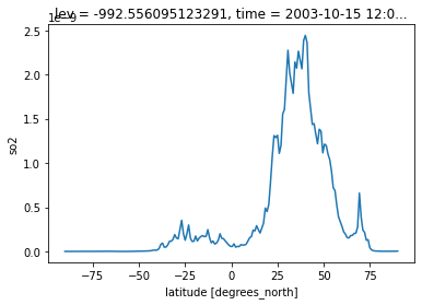
zonal mean and one level and convert to pandas dataframe
%%time
dset_selection = dset['so2'].sel(lev=-1000, method='nearest').mean('lon').load()
CPU times: user 4min 53s, sys: 1min 11s, total: 6min 4s
Wall time: 12min 5s
dset_selection
<xarray.DataArray 'so2' (time: 1980, lat: 192)>
array([[4.4148924e-11, 4.3374932e-11, 4.1744469e-11, ..., 2.0261100e-12,
        1.8938171e-12, 1.8695366e-12],
       [3.1989539e-11, 3.1808257e-11, 3.1800659e-11, ..., 1.2741638e-12,
        1.2158472e-12, 1.1790553e-12],
       [2.9416582e-12, 2.6269848e-12, 2.5257598e-12, ..., 6.3785300e-13,
        6.2758875e-13, 6.3872253e-13],
       ...,
       [8.3957434e-13, 8.9930792e-13, 8.8156679e-13, ..., 4.1710988e-12,
        4.0890802e-12, 5.4941021e-12],
       [7.7786545e-12, 7.8954681e-12, 8.0431321e-12, ..., 2.4857640e-11,
        2.7402766e-11, 3.3165942e-11],
       [1.2275407e-11, 1.2175271e-11, 1.2504974e-11, ..., 4.6298299e-10,
        4.6481125e-10, 4.7047843e-10]], dtype=float32)
Coordinates:
  * lat        (lat) float64 -90.0 -89.06 -88.12 -87.17 ... 88.12 89.06 90.0
    lev        float64 -992.6
  * time       (time) object 1850-01-15 12:00:00 ... 2014-12-15 12:00:00
    member_id  <U8 'r1i1p1f1'
xarray.DataArray
'so2'
- time: 1980
- lat: 192
- 4.415e-11 4.337e-11 4.174e-11 ... 4.63e-10 4.648e-10 4.705e-10
array([[4.4148924e-11, 4.3374932e-11, 4.1744469e-11, ..., 2.0261100e-12, 1.8938171e-12, 1.8695366e-12], [3.1989539e-11, 3.1808257e-11, 3.1800659e-11, ..., 1.2741638e-12, 1.2158472e-12, 1.1790553e-12], [2.9416582e-12, 2.6269848e-12, 2.5257598e-12, ..., 6.3785300e-13, 6.2758875e-13, 6.3872253e-13], ..., [8.3957434e-13, 8.9930792e-13, 8.8156679e-13, ..., 4.1710988e-12, 4.0890802e-12, 5.4941021e-12], [7.7786545e-12, 7.8954681e-12, 8.0431321e-12, ..., 2.4857640e-11, 2.7402766e-11, 3.3165942e-11], [1.2275407e-11, 1.2175271e-11, 1.2504974e-11, ..., 4.6298299e-10, 4.6481125e-10, 4.7047843e-10]], dtype=float32) - lat(lat)float64-90.0 -89.06 -88.12 ... 89.06 90.0
- axis :
- Y
- bounds :
- lat_bnds
- standard_name :
- latitude
- title :
- Latitude
- type :
- double
- units :
- degrees_north
- valid_max :
- 90.0
- valid_min :
- -90.0
array([-90. , -89.057592, -88.115183, -87.172775, -86.230366, -85.287958, -84.34555 , -83.403141, -82.460733, -81.518325, -80.575916, -79.633508, -78.691099, -77.748691, -76.806283, -75.863874, -74.921466, -73.979058, -73.036649, -72.094241, -71.151832, -70.209424, -69.267016, -68.324607, -67.382199, -66.439791, -65.497382, -64.554974, -63.612565, -62.670157, -61.727749, -60.78534 , -59.842932, -58.900524, -57.958115, -57.015707, -56.073298, -55.13089 , -54.188482, -53.246073, -52.303665, -51.361257, -50.418848, -49.47644 , -48.534031, -47.591623, -46.649215, -45.706806, -44.764398, -43.82199 , -42.879581, -41.937173, -40.994764, -40.052356, -39.109948, -38.167539, -37.225131, -36.282723, -35.340314, -34.397906, -33.455497, -32.513089, -31.570681, -30.628272, -29.685864, -28.743455, -27.801047, -26.858639, -25.91623 , -24.973822, -24.031414, -23.089005, -22.146597, -21.204188, -20.26178 , -19.319372, -18.376963, -17.434555, -16.492147, -15.549738, -14.60733 , -13.664921, -12.722513, -11.780105, -10.837696, -9.895288, -8.95288 , -8.010471, -7.068063, -6.125654, -5.183246, -4.240838, -3.298429, -2.356021, -1.413613, -0.471204, 0.471204, 1.413613, 2.356021, 3.298429, 4.240838, 5.183246, 6.125654, 7.068063, 8.010471, 8.95288 , 9.895288, 10.837696, 11.780105, 12.722513, 13.664921, 14.60733 , 15.549738, 16.492147, 17.434555, 18.376963, 19.319372, 20.26178 , 21.204188, 22.146597, 23.089005, 24.031414, 24.973822, 25.91623 , 26.858639, 27.801047, 28.743455, 29.685864, 30.628272, 31.570681, 32.513089, 33.455497, 34.397906, 35.340314, 36.282723, 37.225131, 38.167539, 39.109948, 40.052356, 40.994764, 41.937173, 42.879581, 43.82199 , 44.764398, 45.706806, 46.649215, 47.591623, 48.534031, 49.47644 , 50.418848, 51.361257, 52.303665, 53.246073, 54.188482, 55.13089 , 56.073298, 57.015707, 57.958115, 58.900524, 59.842932, 60.78534 , 61.727749, 62.670157, 63.612565, 64.554974, 65.497382, 66.439791, 67.382199, 68.324607, 69.267016, 70.209424, 71.151832, 72.094241, 73.036649, 73.979058, 74.921466, 75.863874, 76.806283, 77.748691, 78.691099, 79.633508, 80.575916, 81.518325, 82.460733, 83.403141, 84.34555 , 85.287958, 86.230366, 87.172775, 88.115183, 89.057592, 90. ]) - lev()float64-992.6
- axis :
- Z
- bounds :
- lev_bnds
- positive :
- up
- standard_name :
- alevel
- title :
- atmospheric model level
- type :
- double
- units :
- hPa
array(-992.55609512)
- time(time)object1850-01-15 12:00:00 ... 2014-12-...
- axis :
- T
- bounds :
- time_bnds
- standard_name :
- time
- title :
- time
- type :
- double
array([cftime.DatetimeNoLeap(1850, 1, 15, 12, 0, 0, 0), cftime.DatetimeNoLeap(1850, 2, 14, 0, 0, 0, 0), cftime.DatetimeNoLeap(1850, 3, 15, 12, 0, 0, 0), ..., cftime.DatetimeNoLeap(2014, 10, 15, 12, 0, 0, 0), cftime.DatetimeNoLeap(2014, 11, 15, 0, 0, 0, 0), cftime.DatetimeNoLeap(2014, 12, 15, 12, 0, 0, 0)], dtype=object) - member_id()<U8'r1i1p1f1'
array('r1i1p1f1', dtype='<U8')
dset_selection.sel(time=cftime.DatetimeNoLeap(2003, 10, 15), method="nearest").plot()
[<matplotlib.lines.Line2D at 0x7fd3072a8670>]
Convert to pandas dataframe
%%time
pdf = dset_selection.to_dataframe()
CPU times: user 56.4 ms, sys: 2.27 ms, total: 58.7 ms
Wall time: 85.7 ms
pdf.head()
| lev | member_id | so2 | ||
|---|---|---|---|---|
| time | lat | |||
| 1850-01-15 12:00:00 | -90.000000 | -992.556095 | r1i1p1f1 | 4.414892e-11 |
| -89.057592 | -992.556095 | r1i1p1f1 | 4.337493e-11 | |
| -88.115183 | -992.556095 | r1i1p1f1 | 4.174447e-11 | |
| -87.172775 | -992.556095 | r1i1p1f1 | 4.043559e-11 | |
| -86.230366 | -992.556095 | r1i1p1f1 | 4.044334e-11 |
Drop a column
pdf.drop('member_id', axis=1, inplace=True)
pdf.head()
| lev | so2 | ||
|---|---|---|---|
| time | lat | ||
| 1850-01-15 12:00:00 | -90.000000 | -992.556095 | 4.414892e-11 |
| -89.057592 | -992.556095 | 4.337493e-11 | |
| -88.115183 | -992.556095 | 4.174447e-11 | |
| -87.172775 | -992.556095 | 4.043559e-11 | |
| -86.230366 | -992.556095 | 4.044334e-11 |
Save to local file
pdf.to_csv("CMIP_NCAR_CESM2-WACCM_historical_AERmon_zonal_mean.csv", sep='\t')
Save your results to Remote private object storage
your credentials are in
$HOME/.aws/credentialscheck with your instructor to get the secret access key (replace XXX by the right key)
[default]
aws_access_key_id=forces2021-work
aws_secret_access_key=XXXXXXXXXXXX
aws_endpoint_url=https://forces2021.uiogeo-apps.sigma2.no/
It is important to save your results in a place that can last longer than a few days/weeks!
import s3fs
fsg = s3fs.S3FileSystem(anon=False,
      client_kwargs={
         'endpoint_url': 'https://forces2021.uiogeo-apps.sigma2.no/'
      })
Upload local file to remote storage
s3_path =  "s3://work/annefou/CMIP_NCAR_CESM2-WACCM_historical_AERmon_zonal_mean.csv"
print(s3_path)
s3://work/annefou/CMIP_NCAR_CESM2-WACCM_historical_AERmon_zonal_mean.csv
fsg.put('CMIP_NCAR_CESM2-WACCM_historical_AERmon_zonal_mean.csv', s3_path)