From hybrid sigma-pressure (model) levels to pressure levels
Overview
Teaching: 0 min
Exercises: 0 minQuestions
How to interpolate data to pressure levels?
Objectives
Learn to interpolate data to pressure levels
Interpolate from model levels to pressure levels
Interpolate to one pressure level
PyNGL (Python NCL Graphics Library) is a python interface with the same core graphics as NCL (NCAR Command Language) for visualization and data processing.
In this section we are going to use Ngl.vinth2p.
-
This PyNGL function interpolates CESM hybrid coordinates (i.e., model levels) to pressure coordinates.
-
The type of interpolation is currently a variant of transformed pressure coordinates with the interpolation type specified by intyp.
-
All hybrid coordinate values are transformed to pressure values.
- If the input data (i.e., to be interpolated) is on midlevels, then hyam/hybm coefficients should be supplied;
- If the input data is on interfaces, then hyai/hybi coefficients should be supplied.
Warning
The unit for psrf (the surface pressure at each grid point) is Pascals (Pa) whereas the unit for pnew (lists of output pressure levels) and p0 (scalar value equal to surface reference pressure) is millibars (mb).
# Python package that makes working with labelled multi-dimensional arrays simple and efficient
import Ngl
import os
import xarray as xr
import numpy as np
import cartopy.crs as ccrs
import matplotlib.pyplot as plt
%matplotlib inline
path = 'shared-ns1000k/GEO4962/outputs/runs/F2000climo.f19_g17.control/atm/hist/'
filename = path + 'F2000climo.f19_g17.control.cam.h0.0009-01.nc'
print(filename)
# load netcdf file into an xarray dataset
ds = xr.open_dataset(filename, decode_times=True)
# Extract the desired variables (need numpy arrays for vertical interpolation)
hyam = ds["hyam"]
hybm = ds["hybm"]
T = ds["T"]
psrf = ds["PS"]
P0mb = 0.01*ds["P0"]
lats = ds["lat"]
lons = ds["lon"]
# Define the output pressure levels.
pnew = [850.]
# Do the interpolation.
intyp = 1 # 1=linear, 2=log, 3=log-log
kxtrp = False # True=extrapolate (when the output pressure level is outside of the range of psrf)
# Vertical interpolation
Tnew = Ngl.vinth2p(T,hyam,hybm,pnew,psrf,intyp,P0mb,1,kxtrp)
Tnew[Tnew==1e30] = np.NaN
# Create new xarray Dataset
dset_p = xr.Dataset({'T850': (('lat','lon'), Tnew[0,0,:,:])},
{'lon': lons, 'lat': lats})
dset_p.T850.attrs['units'] = 'K'
dset_p.T850.attrs['long_name'] = "Temperature"
dset_p.T850.attrs['standard_name'] = 'T'
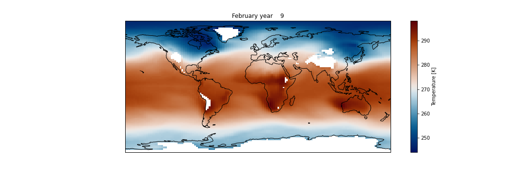
# Plotting
fig = plt.figure(figsize=(15, 5))
ax = plt.axes(projection=ccrs.PlateCarree())
dset_p.T850.plot(ax=ax, transform=ccrs.PlateCarree(), cmap=load_cmap('vik'))
ax.coastlines()
plt.title(ds.time.values[0].strftime("%B year %Y"))
Loading colormaps
In your jupyter notebook, you can load additional/customized colormap using the following statment:
%run shared-ns1000k/GEO4962/scripts/load_cmap.ipynbwith load_cmap.py.
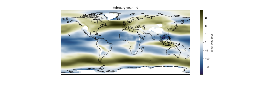
Create a map plot for the zonal wind (U) at 850 mb
Make a similar plot with U, using the same structure and code as for T.
Solution
pnew = [850.]

#  Do the interpolation.
intyp = 1                              # 1=linear, 2=log, 3=log-log
kxtrp = False                          # True=extrapolate (when the output pressure level is outside of the range of psrf)

U    = ds["U"]

UonP = Ngl.vinth2p(U,hyam,hybm,pnew,psrf,intyp,P0mb,1,kxtrp)

ntime, output_levels, nlat, nlon = UonP.shape

UonP[UonP==1e30] = np.NaN

dset_p=xr.Dataset({'U850': (('lat','lon'), UonP[0,0,:,:])},
                  {'lat':  lats, 'lon':  lons})
dset_p.U850.attrs['units'] = 'm/s'
dset_p.U850.attrs['long_name'] = "zonal wind"
dset_p.U850.attrs['standard_name'] = 'U'
fig = plt.figure(figsize=(15, 5))
ax = plt.axes(projection=ccrs.PlateCarree())

dset_p.U850.plot(ax=ax,
           transform=ccrs.PlateCarree(),
           cmap=load_cmap('broc')
           )

ax.coastlines()
plt.title(ds.time.values[0].strftime("%B year %Y"))
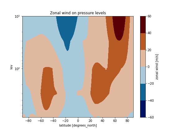
Georeferenced Latitude-Vertical plot on pressure levels
Let’s go back to Georeferenced Latitude-Vertical plots but now we wish the vertical axis to represent pressure levels and not hybrid sigma pressure levels.
We will first plot the zonal wind (U):
import xarray as xr
import numpy as np
import matplotlib.pyplot as plt

pnew = [850., 700., 600, 500., 400., 300., 100., 30., 10.]

intyp = 1                             # 1=linear, 2=log, 3=log-log
kxtrp = True                          # True=extrapolate

UonP = Ngl.vinth2p(U,hyam,hybm,pnew,psrf,intyp,P0mb,1,kxtrp)

ntime, output_levels, nlat, nlon = UonP.shape
You will notice that here we used kxtrp = True in order to extrapolate when the pressure level is outside of the range of psrf (the array of surface pressures).
In this example pnew is an array containing pressure levels and we interpolate U on these levels to generate a new array called UonP.
Then we average UonP along all the longitudes and generate a new array called Umean:
UonP[UonP==1e30] = np.NaN
print(UonP.mean(axis=3).shape,lats.shape)
Umean=xr.Dataset({'U': (('lev','lat'), UonP.mean(axis=3)[0,:,:])},
                 {'lev':  np.asarray(pnew), 'lat':  lats})
Umean.U.attrs['units'] = 'm/s'
Umean.U.attrs['long_name'] = "zonal wind"
Umean.U.attrs['standard_name'] = 'U'
We can now plot Umean:
fig = plt.figure(figsize=(8, 6))
Umean.U.plot.contourf(cmap=load_cmap('vik'))
plt.ylim(plt.ylim()[::-1])
plt.yscale('log')
plt.ylim(top=10.)
plt.ylim(bottom=850.)
plt.title("Zonal wind on pressure levels")
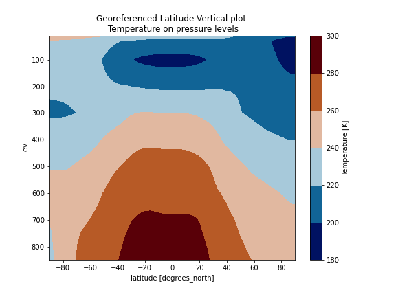
Create a Georeferenced Latitude-Vertical temperature plot on the following pressure levels:
pnew = [850., 700., 600, 500., 400., 300., 100., 30., 10.]
- Try setting
kxtrp = Falseand make another plot withkxtrp = True- What do you observe?
- Is there anything wrong?
Solution
Note: In the plot below we do not use a log scale for the vertical axis in order to highlight the issue with missing values.
import xarray as xr
import numpy as np
import matplotlib.pyplot as plt

pnew = [850., 700., 600, 500., 400., 300., 100., 30., 10.]

intyp = 1                             # 1=linear, 2=log, 3=log-log
kxtrp = True                          # True=extrapolate

Tnew = Ngl.vinth2p(T,hyam,hybm,pnew,psrf,intyp,P0mb,1,kxtrp)

ntime, output_levels, nlat, nlon = Tnew.shape

Tnew[Tnew==1e30] = np.NaN

Tmean=xr.Dataset({'T': (('lev','lat'), Tnew.mean(axis=3)[0,:,:])},
                 {'lev':  np.asarray(pnew), 'lat':  lats})
Tmean.T.attrs['units'] = 'K'
Tmean.T.attrs['long_name'] = "Temperature"
Tmean.T.attrs['standard_name'] = 'T'

fig = plt.figure(figsize=(8, 6))
Tmean.T.plot.contourf(cmap=load_cmap('vik'))
# Invert vertical axis
plt.ylim(plt.ylim()[::-1])
plt.ylim(top=10.)
plt.ylim(bottom=850.)
plt.xlim(left=-90)
plt.xlim(right=90)
plt.title("Georeferenced Latitude-Vertical plot \n Temperature on pressure levels")
Key Points
hybrid sigma levels
pressure levels