You can access your data via the dataset number. Using a Python kernel, you can access dataset number 42 with handle = open(get(42), 'r').
To save data, write your data to a file, and then call put('filename.txt'). The dataset will then be available in your galaxy history.
When using a non-Python kernel, get and put are available as command-line tools, which can be accessed using system calls in R, Julia, and Ruby. For example, to read dataset number 42 into R, you can write handle <- file(system('get -i 42', intern = TRUE)).
To save data in R, write the data to a file and then call system('put -p filename.txt').
Notebooks can be saved to Galaxy by clicking the large green button at the top right of the IPython interface.
More help and informations can be found on the project website.
import xarray as xr
import cartopy.crs as ccrs
import matplotlib.pyplot as plt
import numpy as np
import cftime
import glob
import cdsapi
%matplotlib inline
Adding your CDS API key
- Login to cds
- Visit page How to install the cds api key
- Start a new Terminal Session
- Use
nanoto edit your cds api:
nano $HOME/.cdsapircc = cdsapi.Client()
c.retrieve(
'projections-cmip5-daily-single-levels',
{
'ensemble_member': 'r1i1p1',
'format': 'zip',
'experiment': 'historical',
'variable': '2m_temperature',
'model': 'mpi_esm_lr',
'period': [
'19600101-19691231', '19700101-19791231', '19800101-19891231',
'19900101-19991231', '20000101-20051231',
],
},
'cmip5_mpi_esm_lr_daily_t2m.zip')
# Save data into Galaxy history
!put -p cmip5_mpi_esm_lr_daily_t2m.zip -t zip
!mkdir -p mpi_daily_h
!cd mpi_daily_h && unzip ../cmip5_mpi_esm_lr_daily_t2m.zip
filenames = glob.glob('mpi_daily_h/tas_*_MPI-ESM-LR_*.nc')
print(filenames)
dset = xr.open_mfdataset(filenames, decode_times=True, use_cftime=True, combine='by_coords')
dset
p = dset['tas'].loc['1961-01-01':'2005-12-31'].sel(lat=46.5,lon=13.8, method="nearest")
mean_mpi_1961_2005 = p.mean().values
std_mpi_1961_2005 = p.std().values
print(mean_mpi_1961_2005, std_mpi_1961_2005)
!wget http://berkeleyearth.lbl.gov/auto/Stations/TAVG/Text/22498-TAVG-Data.txt
# Save data into Galaxy history
!put -p 22498-TAVG-Data.txt -t txt
import pandas as pd
filename = '22498-TAVG-Data.txt'
data = pd.read_csv(filename, sep='\s+', header=None, comment='%')
mean_st_1961_2005 = data[(data[0] >= 1961 ) & (data[0] <= 2005)][6].mean()
std_st_1961_2005 = data[(data[0] >= 1961 ) & (data[0] <= 2005)][6].std()
print(mean_st_1961_2005 + 273.15, std_st_1961_2005)
dset.close()
- We now have mean temperature and standard deviation for both MPI-ESM-LR historical and RATECE-PLANICA Slovenia meteorological station. These values will be used for our bias correction
c.retrieve(
    'projections-cmip5-daily-single-levels',
    {
        'ensemble_member': 'r1i1p1',
        'format': 'zip',
        'experiment': 'historical',
        'variable': [
            'maximum_2m_temperature_in_the_last_24_hours', 'minimum_2m_temperature_in_the_last_24_hours',
        ],
        'model': 'mpi_esm_lr',
        'period': [
            '19600101-19691231', '19700101-19791231', '19800101-19891231',
            '19900101-19991231', '20000101-20051231',
        ],
    },
    'cmip5_mpi_esm_lr_daily_tasmin_tasmax.zip')
# Save data into Galaxy history
!put -p cmip5_mpi_esm_lr_daily_tasmin_tasmax.zip -t zip
!mkdir -p mpi_daily_h
!cd mpi_daily_h && unzip ../cmip5_mpi_esm_lr_daily_tasmin_tasmax.zip && rm ../cmip5_mpi_esm_lr_daily_tasmin_tasmax.zip
filenames = glob.glob('mpi_daily_h/tas*_MPI-ESM-LR_*.nc')
print(filenames)
dset_hist = xr.open_mfdataset(filenames, decode_times=True, use_cftime=True, combine='by_coords')
p = dset_hist['tasmin'].loc['1961-01-01':'2005-12-31'].sel(lat=46.5,lon=13.8, method="nearest")
t2min_h_bias_corrected = (p - mean_mpi_1961_2005)/std_mpi_1961_2005 * std_st_1961_2005 + mean_st_1961_2005
p = dset_hist['tasmax'].loc['1961-01-01':'2005-12-31'].sel(lat=46.5,lon=13.8, method="nearest")
t2max_h_bias_corrected = (p - mean_mpi_1961_2005)/std_mpi_1961_2005 * std_st_1961_2005 + mean_st_1961_2005
t2max_h_bias_corrected.sel(time = t2max_h_bias_corrected.time.dt.year.isin([1970, 1970])).plot()
t2min_h_bias_corrected.sel(time = t2min_h_bias_corrected.time.dt.year.isin([1970, 1970])).plot()
c.retrieve(
    'projections-cmip5-daily-single-levels',
    {
        'ensemble_member': 'r1i1p1',
        'format': 'zip',
        'experiment': 'rcp_8_5',
        'variable': [
            'maximum_2m_temperature_in_the_last_24_hours', 'minimum_2m_temperature_in_the_last_24_hours',
        ],
        'area' : "47.5/12/44.5/14", #N/W/S/E
        'model': 'mpi_esm_lr',
        'period': [
            '20400101-20491231', '20500101-20591231', '20600101-20691231',
            '20700101-20791231', '20800101-20891231', '20900101-21001231',
        ],
    },
    'cmip5_mpi_esm_lr_daily_tasmin_tasmax_proj.zip')
!mkdir -p mpi_daily_p
!cd mpi_daily_p && unzip ../cmip5_mpi_esm_lr_daily_tasmin_tasmax_proj.zip && rm ../cmip5_mpi_esm_lr_daily_tasmin_tasmax_proj.zip
filenames = glob.glob('mpi_daily_p/tas*_MPI-ESM-LR_*.nc')
print(filenames)
dset_p = xr.open_mfdataset(filenames, decode_times=True, use_cftime=True, combine='by_coords')
p = dset_p['tasmin'].loc['2040-01-01':'2100-12-31'].sel(lat=46.5,lon=13.8, method="nearest")
t2min_p_bias_corrected = (p - mean_mpi_1961_2005)/std_mpi_1961_2005 * std_st_1961_2005 + mean_st_1961_2005
p = dset_p['tasmax'].loc['2040-01-01':'2100-12-31'].sel(lat=46.5,lon=13.8, method="nearest")
t2max_p_bias_corrected = (p - mean_mpi_1961_2005)/std_mpi_1961_2005 * std_st_1961_2005 + mean_st_1961_2005
nb_favourable_h = t2min_h_bias_corrected.where((t2min_h_bias_corrected < 0) & (t2max_h_bias_corrected <= 3)).groupby('time.year').count()
nb_favourable_h
nb_favourable_p = t2min_p_bias_corrected.where((t2min_p_bias_corrected < 0) & (t2max_p_bias_corrected <= 3)).groupby('time.year').count()
nb_favourable_p
nb_favourable = xr.merge([nb_favourable_h, nb_favourable_p])
nb_favourable
series = nb_favourable.tasmin.to_series()
series.index = pd.to_datetime(series.index,  format='%Y')
series.head()
import numpy as np
series.loc[(series.index.year > 2000) & (series.index.year <= 2005)] = np.nan
series.loc[(series.index.year == 2040)] = np.nan
series.head(50)
series10YS = series.groupby(pd.Grouper(freq='10YS')).mean()
import matplotlib.pyplot as plt
from datetime import datetime
from datetime import timedelta
from dateutil.relativedelta import relativedelta
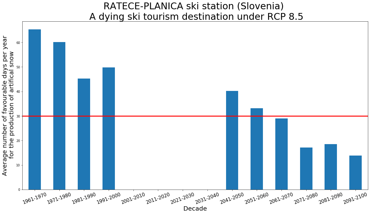
fig = plt.figure(1, figsize=[20,10])
ax = plt.subplot(1, 1, 1)
series10YS.plot.bar(ax=ax)
plt.axhline(y=30, color='r', linestyle='-', linewidth=3)
labels = [datetime.strptime(item.get_text(), '%Y-%m-%d %H:%M:%S').strftime("%Y") + '-' +
(datetime.strptime(item.get_text() , '%Y-%m-%d %H:%M:%S') + relativedelta(years=9)).strftime("%Y") for item in ax.get_xticklabels()]
ax.set_xticklabels(labels, rotation=20, fontsize = 15)
ax.set_xlabel('Decade', fontsize = 20)
ax.set_ylabel('Average number of favourable days per year\n for the production of artifical snow', fontsize = 20)
plt.title("RATECE-PLANICA ski station (Slovenia) \n A dying ski tourism destination under RCP 8.5", fontsize=30)