Working with Pandas dataframes
Overview
Teaching: 0 min
Exercises: 0 minQuestions
What is Pandas?
How can I import data with Pandas?
Why should I use Pandas to work with data?
How can I access specific data within my data set?
How can Python and Pandas help me to analyse my data?
Objectives
What is Pandas? Getting started with pandas
To analyze data, we like to use two-dimensional tables – like in SQL and in Excel. Originally, Python didn’t have this feature. But that’s why Pandas is so important! I like to say, Pandas is the “SQL of Python.” Pandas is the library that will help us to handle two-dimensional data tables in Python. In many senses it’s really similar to SQL, though.
Why should I use Pandas to work with data?
Because:
- handle headings better than with Numpy
- Pandas Series and DataFrame are also Numpy arrays
- provide some clarity in your data
- especially important if you work with time series as you can downscale and upscale your data based on the time series
Essential functions
Top 20 most popular pandas function on GitHub (in 2016) https://galeascience.wordpress.com/2016/08/10/top-10-pandas-numpy-and-scipy-functions-on-github/
import pandas as pd
import numpy as np
How can I import data with Pandas?
- Array can be created as in Numpy (Series)
- Data can be imported from text files (.csv, .txt and other type of text formats) or directly from excel files (DataFrames)
Series
One-dimensional array-like object (very similar to Numpy 1-D arrays). pd.Series is characterized by an index and a single column.
temperature_Oslo = pd.Series([4, 6, 6, 9, 8, 7, 8]) # temperature in the middle of the day at Blindern for the next 7 days

temperature_Oslo
0    4
1    6
2    6
3    9
4    8
5    7
6    8
dtype: int64
By default, the index starts at 0 and stop at the last value in your pd.Series dataset
temperature_Oslo.index # same as range(7) or np.arange(7)
RangeIndex(start=0, stop=7, step=1)
The index can be modified by accessing the index key pd.Series.index
# indexes can be later modified by doing
temperature_Oslo.index = ['Monday', 'Tuesday', 'Wednesday', 'Thursday', 'Friday', 'Saturday', 'Sunday']
temperature_Oslo.index
Index(['Monday', 'Tuesday', 'Wednesday', 'Thursday', 'Friday', 'Saturday',
       'Sunday'],
      dtype='object')
The easiest way to create a pd.Series is to define a dictionnary and pass it to the pd.Series
ndata = {'Monday' : 4 , 'Tuesday' : 6 , 'Wednesday' : 6 , 'Thursday' : 9 , 'Friday' : 8 , 'Saturday' : 7, 'Sunday' : 8}


# feed pd.Series the previously created dictionary
temperature_Oslo = pd.Series(ndata)

# print the data on the screen
temperature_Oslo
Monday       4
Tuesday      6
Wednesday    6
Thursday     9
Friday       8
Saturday     7
Sunday       8
dtype: int64
Values within the pd.Series can be accessed either by pd.Series[variable] or pd.Series.variable
# change in temperature between Monday and Tuesday
print (temperature_Oslo['Monday'] - temperature_Oslo['Tuesday'])

# similar to
print (temperature_Oslo.Monday - temperature_Oslo.Tuesday)
-2
-2
DataFrame
DataFrame is the most popular function used in Pandas. Help to deal with large rectangular datasets. There are many ways to construct a DataFrame, and can mostly be separated in two groups:
- Manually, by specifying a dictionary containing a string (the header) and a list of numbers or strings
- Importing a text or excel file, which contains a x number of data
Creating a DataFrame manually
We can again make us of dictionnary variables but this time we will have a dataset with a multiple number of columns
data = {'Day of the week' : ['Monday', 'Tuesday', 'Wednesday', 'Thursday', 'Friday', 'Saturday', 'Sunday'],
        'Temperature in the middle of the day' : [4, 6, 6, 9, 8, 7, 8],
        'Wind (m/s)' : [1, 6, 2, 2, 4, 3, 3],
        'Weather conditions' : ['Cloud & Sun', 'Cloud', 'Cloud', 'Cloud & Sun', 'Cloud & Sun', 'Sun', 'Cloud']}

frame = pd.DataFrame(data)

frame
| Day of the week | Temperature in the middle of the day | Wind (m/s) | Weather conditions | |
|---|---|---|---|---|
| 0 | Monday | 4 | 1 | Cloud & Sun |
| 1 | Tuesday | 6 | 6 | Cloud |
| 2 | Wednesday | 6 | 2 | Cloud |
| 3 | Thursday | 9 | 2 | Cloud & Sun |
| 4 | Friday | 8 | 4 | Cloud & Sun |
| 5 | Saturday | 7 | 3 | Sun |
| 6 | Sunday | 8 | 3 | Cloud |
Interesting functionalities and how can I access specific data within my data set?
frame.head() # print the first five rows
| depth (m) | Age_04032019_0,1mm_0,01yr | Age. Cal. CE | Al | Si | P | S | Cl | Ar | K | ... | Si/Ti | P/Ti | Fe/Mn | Fe/Ti | Pb/Ti | S/OM | S/Ti | Hg/Mn | Hg/Ti.1 | Hg/MO | |
|---|---|---|---|---|---|---|---|---|---|---|---|---|---|---|---|---|---|---|---|---|---|
| 0 | 0.0000 | -68.00 | 2018.00 | 25 | 11 | 12 | 82 | 29 | 136 | 6 | ... | 0.137500 | 0.150000 | 80.225806 | 62.175000 | 0.0 | 11.958182 | 1.025000 | 0.000000 | 0.000000 | 0.000000 |
| 1 | 0.0002 | -67.97 | 2017.97 | 22 | 0 | 18 | 76 | 23 | 167 | 19 | ... | 0.000000 | 0.500000 | 98.203704 | 147.305556 | 0.0 | 10.919643 | 2.111111 | 3.092593 | 4.638889 | 23.994480 |
| 2 | 0.0004 | -67.81 | 2017.81 | 53 | 6 | 0 | 37 | 9 | 141 | 19 | ... | 0.272727 | 0.000000 | 92.290323 | 260.090909 | 0.0 | 5.525249 | 1.681818 | 0.274194 | 0.772727 | 2.538628 |
| 3 | 0.0006 | -67.65 | 2017.65 | 18 | 6 | 17 | 64 | 8 | 167 | 23 | ... | 0.157895 | 0.447368 | 138.069767 | 156.236842 | 0.0 | 9.239006 | 1.684211 | 0.000000 | 0.000000 | 0.000000 |
| 4 | 0.0008 | -67.57 | 2017.57 | 36 | 32 | 22 | 74 | 13 | 129 | 23 | ... | 0.323232 | 0.222222 | 75.576471 | 64.888889 | 0.0 | 10.632997 | 0.747475 | 1.000000 | 0.858586 | 12.213577 |
5 rows × 45 columns
print (frame.columns) # print name of the columns
Index(['Day of the week', 'Temperature in the middle of the day', 'Wind (m/s)',
       'Weather conditions'],
      dtype='object')
Apply numpy functions to pandas arrays
np.mean(frame['Temperature in the middle of the day'])
6.857142857142857
Switch columns in the DataFrame
pd.DataFrame(data, columns=['Day of the week', 'Weather conditions', 'Temperature in the middle of the day', 'Wind (m/s)'])
| Day of the week | Weather conditions | Temperature in the middle of the day | Wind (m/s) | |
|---|---|---|---|---|
| 0 | Monday | Cloud & Sun | 4 | 1 |
| 1 | Tuesday | Cloud | 6 | 6 |
| 2 | Wednesday | Cloud | 6 | 2 |
| 3 | Thursday | Cloud & Sun | 9 | 2 |
| 4 | Friday | Cloud & Sun | 8 | 4 |
| 5 | Saturday | Sun | 7 | 3 |
| 6 | Sunday | Cloud | 8 | 3 |
Locate row based on your index
print (frame.loc[0])

print (frame.loc[6])
Day of the week                              Monday
Temperature in the middle of the day              4
Wind (m/s)                                        1
Weather conditions                      Cloud & Sun
Name: 0, dtype: object
Day of the week                         Sunday
Temperature in the middle of the day         8
Wind (m/s)                                   3
Weather conditions                       Cloud
Name: 6, dtype: object
Assign values in the DataFrame
# we create a new DataFrame with a new column
nframe = pd.DataFrame(data, columns=['Day of the week', 'Weather conditions', 'Temperature in the middle of the day',
                                     'Wind (m/s)', 'Precipitation (mm)'])

nframe
| Day of the week | Weather conditions | Temperature in the middle of the day | Wind (m/s) | Precipitation (mm) | |
|---|---|---|---|---|---|
| 0 | Monday | Cloud & Sun | 4 | 1 | NaN |
| 1 | Tuesday | Cloud | 6 | 6 | NaN |
| 2 | Wednesday | Cloud | 6 | 2 | NaN |
| 3 | Thursday | Cloud & Sun | 9 | 2 | NaN |
| 4 | Friday | Cloud & Sun | 8 | 4 | NaN |
| 5 | Saturday | Sun | 7 | 3 | NaN |
| 6 | Sunday | Cloud | 8 | 3 | NaN |
Modify a single value
nframe['Precipitation (mm)'].values[0] = 2.3

nframe
| Day of the week | Weather conditions | Temperature in the middle of the day | Wind (m/s) | Precipitation (mm) | |
|---|---|---|---|---|---|
| 0 | Monday | Cloud & Sun | 4 | 1 | 2.3 |
| 1 | Tuesday | Cloud | 6 | 6 | NaN |
| 2 | Wednesday | Cloud | 6 | 2 | NaN |
| 3 | Thursday | Cloud & Sun | 9 | 2 | NaN |
| 4 | Friday | Cloud & Sun | 8 | 4 | NaN |
| 5 | Saturday | Sun | 7 | 3 | NaN |
| 6 | Sunday | Cloud | 8 | 3 | NaN |
Modify a slice of values
nframe['Precipitation (mm)'].values[1:4] = 1.0

nframe
| Day of the week | Weather conditions | Temperature in the middle of the day | Wind (m/s) | Precipitation (mm) | |
|---|---|---|---|---|---|
| 0 | Monday | Cloud & Sun | 4 | 1 | 2.3 |
| 1 | Tuesday | Cloud | 6 | 6 | 1 |
| 2 | Wednesday | Cloud | 6 | 2 | 1 |
| 3 | Thursday | Cloud & Sun | 9 | 2 | 1 |
| 4 | Friday | Cloud & Sun | 8 | 4 | NaN |
| 5 | Saturday | Sun | 7 | 3 | NaN |
| 6 | Sunday | Cloud | 8 | 3 | NaN |
Change all values
nframe['Precipitation (mm)'] = 0.0 #equivalent to nframe['Precipitation (mm)'].values[:] = 0.0

nframe
| Day of the week | Weather conditions | Temperature in the middle of the day | Wind (m/s) | Precipitation (mm) | |
|---|---|---|---|---|---|
| 0 | Monday | Cloud & Sun | 4 | 1 | 0.0 |
| 1 | Tuesday | Cloud | 6 | 6 | 0.0 |
| 2 | Wednesday | Cloud | 6 | 2 | 0.0 |
| 3 | Thursday | Cloud & Sun | 9 | 2 | 0.0 |
| 4 | Friday | Cloud & Sun | 8 | 4 | 0.0 |
| 5 | Saturday | Sun | 7 | 3 | 0.0 |
| 6 | Sunday | Cloud | 8 | 3 | 0.0 |
Indexing, reindexing, selection with loc and iloc
nframe = nframe.set_index('Day of the week')

nframe
| Weather conditions | Temperature in the middle of the day | Wind (m/s) | Precipitation (mm) | |
|---|---|---|---|---|
| Day of the week | ||||
| Monday | Cloud & Sun | 4 | 1 | NaN |
| Tuesday | Cloud | 6 | 6 | NaN |
| Wednesday | Cloud | 6 | 2 | NaN |
| Thursday | Cloud & Sun | 9 | 2 | NaN |
| Friday | Cloud & Sun | 8 | 4 | NaN |
| Saturday | Sun | 7 | 3 | NaN |
| Sunday | Cloud | 8 | 3 | NaN |
nframe.loc['Monday']
Weather conditions                      Cloud & Sun
Temperature in the middle of the day              4
Wind (m/s)                                        1
Precipitation (mm)                              NaN
Name: Monday, dtype: object
nframe.iloc[0]
Weather conditions                      Cloud & Sun
Temperature in the middle of the day              4
Wind (m/s)                                        1
Precipitation (mm)                              NaN
Name: Monday, dtype: object
# re-indexing
nframe2 = nframe.reindex(['Wednesday', 'Thursday', 'Friday', 'Saturday', 'Sunday','Monday', 'Tuesday'])

nframe2
| Weather conditions | Temperature in the middle of the day | Wind (m/s) | Precipitation (mm) | |
|---|---|---|---|---|
| Day of the week | ||||
| Wednesday | Cloud | 6 | 2 | NaN |
| Thursday | Cloud & Sun | 9 | 2 | NaN |
| Friday | Cloud & Sun | 8 | 4 | NaN |
| Saturday | Sun | 7 | 3 | NaN |
| Sunday | Cloud | 8 | 3 | NaN |
| Monday | Cloud & Sun | 4 | 1 | NaN |
| Tuesday | Cloud | 6 | 6 | NaN |
Sorting of columns
Sort by a column
nframe2.sort_values(by='Temperature in the middle of the day') #default ascending
| Weather conditions | Temperature in the middle of the day | Wind (m/s) | Precipitation (mm) | |
|---|---|---|---|---|
| Day of the week | ||||
| Monday | Cloud & Sun | 4 | 1 | NaN |
| Wednesday | Cloud | 6 | 2 | NaN |
| Tuesday | Cloud | 6 | 6 | NaN |
| Saturday | Sun | 7 | 3 | NaN |
| Friday | Cloud & Sun | 8 | 4 | NaN |
| Sunday | Cloud | 8 | 3 | NaN |
| Thursday | Cloud & Sun | 9 | 2 | NaN |
nframe2.sort_values(by='Temperature in the middle of the day', ascending=False) #descending
| Weather conditions | Temperature in the middle of the day | Wind (m/s) | Precipitation (mm) | |
|---|---|---|---|---|
| Day of the week | ||||
| Thursday | Cloud & Sun | 9 | 2 | NaN |
| Friday | Cloud & Sun | 8 | 4 | NaN |
| Sunday | Cloud | 8 | 3 | NaN |
| Saturday | Sun | 7 | 3 | NaN |
| Wednesday | Cloud | 6 | 2 | NaN |
| Tuesday | Cloud | 6 | 6 | NaN |
| Monday | Cloud & Sun | 4 | 1 | NaN |
Sorting by multiple columns
nframe2.sort_values(by=['Temperature in the middle of the day', 'Wind (m/s)'], ascending=False) #descending
| Weather conditions | Temperature in the middle of the day | Wind (m/s) | Precipitation (mm) | |
|---|---|---|---|---|
| Day of the week | ||||
| Thursday | Cloud & Sun | 9 | 2 | NaN |
| Friday | Cloud & Sun | 8 | 4 | NaN |
| Sunday | Cloud | 8 | 3 | NaN |
| Saturday | Sun | 7 | 3 | NaN |
| Tuesday | Cloud | 6 | 6 | NaN |
| Wednesday | Cloud | 6 | 2 | NaN |
| Monday | Cloud & Sun | 4 | 1 | NaN |
Importing a DataFrame
Data is provided by Manon
path = '../data/Manon/' #directory to the file we would like to import
filename = 'data_manon_python.xlsx'  # filename

frame = pd.read_excel(path + filename)

frame.head()
| depth (m) | Age_04032019_0,1mm_0,01yr | Age. Cal. CE | Al | Si | P | S | Cl | Ar | K | ... | Si/Ti | P/Ti | Fe/Mn | Fe/Ti | Pb/Ti | S/OM | S/Ti | Hg/Mn | Hg/Ti.1 | Hg/MO | |
|---|---|---|---|---|---|---|---|---|---|---|---|---|---|---|---|---|---|---|---|---|---|
| 0 | 0.0000 | -68.00 | 2018.00 | 25 | 11 | 12 | 82 | 29 | 136 | 6 | ... | 0.137500 | 0.150000 | 80.225806 | 62.175000 | 0.0 | 11.958182 | 1.025000 | 0.000000 | 0.000000 | 0.000000 |
| 1 | 0.0002 | -67.97 | 2017.97 | 22 | 0 | 18 | 76 | 23 | 167 | 19 | ... | 0.000000 | 0.500000 | 98.203704 | 147.305556 | 0.0 | 10.919643 | 2.111111 | 3.092593 | 4.638889 | 23.994480 |
| 2 | 0.0004 | -67.81 | 2017.81 | 53 | 6 | 0 | 37 | 9 | 141 | 19 | ... | 0.272727 | 0.000000 | 92.290323 | 260.090909 | 0.0 | 5.525249 | 1.681818 | 0.274194 | 0.772727 | 2.538628 |
| 3 | 0.0006 | -67.65 | 2017.65 | 18 | 6 | 17 | 64 | 8 | 167 | 23 | ... | 0.157895 | 0.447368 | 138.069767 | 156.236842 | 0.0 | 9.239006 | 1.684211 | 0.000000 | 0.000000 | 0.000000 |
| 4 | 0.0008 | -67.57 | 2017.57 | 36 | 32 | 22 | 74 | 13 | 129 | 23 | ... | 0.323232 | 0.222222 | 75.576471 | 64.888889 | 0.0 | 10.632997 | 0.747475 | 1.000000 | 0.858586 | 12.213577 |
5 rows × 45 columns
import matplotlib.pyplot as plt
from matplotlib.gridspec import GridSpec
%matplotlib inline
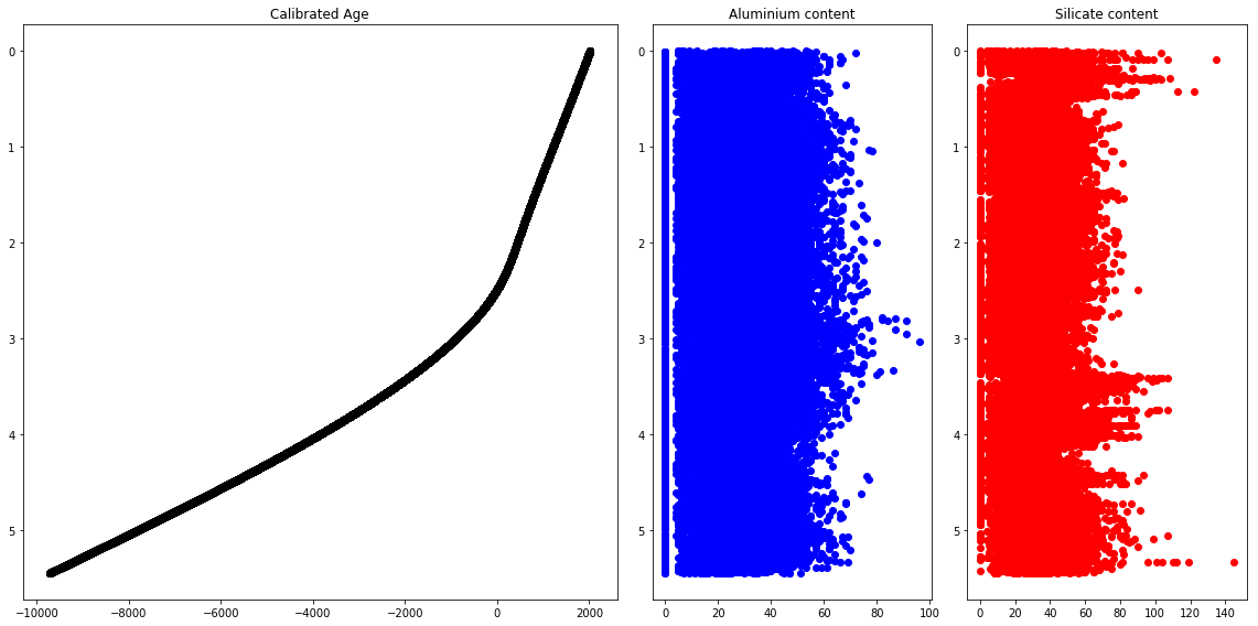
fig = plt.figure(figsize=(16,8))
gs=GridSpec(2,4) # 2 rows, 4 columns
ax1=fig.add_subplot(gs[:,:2]) # Span all rows, firs two columns
ax2=fig.add_subplot(gs[:,2]) # Span all rows, third column
ax3=fig.add_subplot(gs[:,3]) # Span all rows, fourth column
ax1.set_title('Calibrated Age')
ax2.set_title('Aluminium content')
ax3.set_title('Silicate content')
ax1.plot(frame['Age. Cal. CE'],frame['depth (m)'],"ko")
ax1.set_ylim(ax1.get_ylim()[::-1])
ax2.plot(frame['Al'],frame['depth (m)'],"bo")
ax2.set_ylim(ax2.get_ylim()[::-1])
ax3.plot(frame['Si'],frame['depth (m)'],"ro")
ax3.set_ylim(ax3.get_ylim()[::-1])
fig.tight_layout()
Time series
For some of you, most of your data are time series. Time series can be differentiated in two main groups:
- Fixed periods, such as a dataset where you will have data once a day (daily)
- Intervals of time, i.e, discontinuous periods, indicated by a start and end time
we will here see how you can work with timeseries in Pandas
Most important is to have a date format that will be recognized by Python!
Date format
from datetime import datetime

now = datetime.now()

now
datetime.datetime(2019, 3, 31, 12, 37, 38, 694910)
now.year, now.month, now.day
(2019, 3, 31)
Convertion between String and Datetime
More information about the different datetime format can be found here: http://strftime.org/
Most commonly used functions are within the datetime and dateutil modules
Date to string format
timestamp = datetime(2019, 1, 1) # date format

str(timestamp) # string format
'2019-01-01 00:00:00'
timestamp.strftime('%Y-%m-%d') # string format
'2019-01-01'
String to date format
timestamp_str = '2019/04/01'

datetime.strptime(timestamp_str, '%Y/%m/%d')
datetime.datetime(2019, 4, 1, 0, 0)
parse is also a handy function to convert string to date format
Here are few examples:
from dateutil.parser import parse

parse('2019/04/01')
datetime.datetime(2019, 4, 1, 0, 0)
parse('01/04/2019', dayfirst=True) # day in front
datetime.datetime(2019, 4, 1, 0, 0)
In most cases we will work with intervals of date (either continuous or discontinuous).
The easiest case is for continuous measurements as the integrated function pd.date_range can be used
pd.date_range?
dates_2019 = pd.date_range(start='2019/01/01', end='2019/04/01') # default is daily data

dates_2019
DatetimeIndex(['2019-01-01', '2019-01-02', '2019-01-03', '2019-01-04',
               '2019-01-05', '2019-01-06', '2019-01-07', '2019-01-08',
               '2019-01-09', '2019-01-10', '2019-01-11', '2019-01-12',
               '2019-01-13', '2019-01-14', '2019-01-15', '2019-01-16',
               '2019-01-17', '2019-01-18', '2019-01-19', '2019-01-20',
               '2019-01-21', '2019-01-22', '2019-01-23', '2019-01-24',
               '2019-01-25', '2019-01-26', '2019-01-27', '2019-01-28',
               '2019-01-29', '2019-01-30', '2019-01-31', '2019-02-01',
               '2019-02-02', '2019-02-03', '2019-02-04', '2019-02-05',
               '2019-02-06', '2019-02-07', '2019-02-08', '2019-02-09',
               '2019-02-10', '2019-02-11', '2019-02-12', '2019-02-13',
               '2019-02-14', '2019-02-15', '2019-02-16', '2019-02-17',
               '2019-02-18', '2019-02-19', '2019-02-20', '2019-02-21',
               '2019-02-22', '2019-02-23', '2019-02-24', '2019-02-25',
               '2019-02-26', '2019-02-27', '2019-02-28', '2019-03-01',
               '2019-03-02', '2019-03-03', '2019-03-04', '2019-03-05',
               '2019-03-06', '2019-03-07', '2019-03-08', '2019-03-09',
               '2019-03-10', '2019-03-11', '2019-03-12', '2019-03-13',
               '2019-03-14', '2019-03-15', '2019-03-16', '2019-03-17',
               '2019-03-18', '2019-03-19', '2019-03-20', '2019-03-21',
               '2019-03-22', '2019-03-23', '2019-03-24', '2019-03-25',
               '2019-03-26', '2019-03-27', '2019-03-28', '2019-03-29',
               '2019-03-30', '2019-03-31', '2019-04-01'],
              dtype='datetime64[ns]', freq='D')
For discontinuous measurements, you have to build your own list of dates either:
- manually
- or by importing your datasets with specific timestamps
list_of_dates = ['01/01/2019', '19/01/2019', '25/02/2019', '07/03/2019', '01/04/2019'] # day-first european style


converted_list_of_dates = [parse(x, dayfirst=True) for x in list_of_dates]

converted_list_of_dates
[datetime.datetime(2019, 1, 1, 0, 0),
 datetime.datetime(2019, 1, 19, 0, 0),
 datetime.datetime(2019, 2, 25, 0, 0),
 datetime.datetime(2019, 3, 7, 0, 0),
 datetime.datetime(2019, 4, 1, 0, 0)]
Let’s work with the data Manon provided where a calibrated age frame['Age. Cal. CE'] is available
frame['Age. Cal. CE'].head() #print the first 5 values
0    2018.00
1    2017.97
2    2017.81
3    2017.65
4    2017.57
Name: Age. Cal. CE, dtype: float64
We need to transform this column into a date format pandas will familiar with
There are several ways of doing that!
Extracting the year
years = np.floor(frame['Age. Cal. CE'].values)

years
array([ 2018., 2017., 2017., ..., -9718., -9719., -9720.])
years = years.astype('int')

years_str = years.astype('str')

years_str
array(['2018', '2017', '2017', ..., '-9718', '-9719', '-9720'],
      dtype='<U11')
Extracting the month and the day
months_and_days = frame['Age. Cal. CE'].values - years

months_and_days
array([0. , 0.97, 0.81, ..., 0.62, 0.76, 0.91])
months_and_days2 = np.round(months_and_days * 365.25)
months_and_days3 = months_and_days2.astype('int') # integer
months_and_days3
array([ 0, 354, 296, ..., 226, 278, 332])
# set 0 equal to 1 (avoid problem with day of the year = 0)
months_and_days3[months_and_days3 < 1] = 1

months_and_days3
array([ 1, 354, 296, ..., 226, 278, 332])
months_and_days_str = months_and_days3.astype('str')
months_and_days_str
array(['1', '354', '296', ..., '226', '278', '332'], dtype='<U11')
tmp_date = years_str[0].zfill(4) + "/" + months_and_days_str[0].zfill(3) #zfill write 331 as 0331

tmp_date
'2018/001'
datetime_viking = [] # create an empty list

# need to loop through the numpy array
for ix, dates_i in np.ndenumerate(months_and_days_str): #loop through strings

    # we save only the dates before Jesus
    if years[ix] > 0: #datetime does not support negative years or BC dates, need to work with Julian date format?
        tmp_date = years_str[ix].zfill(4) + "/" + months_and_days_str[ix].zfill(3)

        # save to originally empty list
        datetime_viking.append(datetime.strptime(tmp_date, '%Y/%j'))

datetime_viking[:5] # print first five dates
[datetime.datetime(2018, 1, 1, 0, 0),
 datetime.datetime(2017, 12, 20, 0, 0),
 datetime.datetime(2017, 10, 23, 0, 0),
 datetime.datetime(2017, 8, 25, 0, 0),
 datetime.datetime(2017, 7, 27, 0, 0)]
# need to convert to pandas datetime (datetime_viking is a list while we need to work with pandas or numpy array)

# empty panda series
date_pandas = pd.Series([])

#need to use period if we want to work with period younger than 1677

for ix, datev in enumerate(datetime_viking):

    date_tmp = pd.Period(year= datetime_viking[ix].year, month =datetime_viking[ix].month, day = datetime_viking[ix].day, freq='D')
    #print (date_tmp)
    date_pandas = date_pandas.append(pd.Series([date_tmp]))

date_pandas.head()
0    2018-01-01
0    2017-12-20
0    2017-10-23
0    2017-08-25
0    2017-07-27
dtype: period[D]
# we need to create a new data frame containing only data before JC
frame_shortened = frame.iloc[0:len(datetime_viking)]

# and we set the dates as index
frame_shortened.index = date_pandas

# let's have a look at the dataframe
frame_shortened.head()
| depth (m) | Age_04032019_0,1mm_0,01yr | Age. Cal. CE | Al | Si | P | S | Cl | Ar | K | ... | Si/Ti | P/Ti | Fe/Mn | Fe/Ti | Pb/Ti | S/OM | S/Ti | Hg/Mn | Hg/Ti.1 | Hg/MO | |
|---|---|---|---|---|---|---|---|---|---|---|---|---|---|---|---|---|---|---|---|---|---|
| 2018-01-01 | 0.0000 | -68.00 | 2018.00 | 25 | 11 | 12 | 82 | 29 | 136 | 6 | ... | 0.137500 | 0.150000 | 80.225806 | 62.175000 | 0.0 | 11.958182 | 1.025000 | 0.000000 | 0.000000 | 0.000000 |
| 2017-12-20 | 0.0002 | -67.97 | 2017.97 | 22 | 0 | 18 | 76 | 23 | 167 | 19 | ... | 0.000000 | 0.500000 | 98.203704 | 147.305556 | 0.0 | 10.919643 | 2.111111 | 3.092593 | 4.638889 | 23.994480 |
| 2017-10-23 | 0.0004 | -67.81 | 2017.81 | 53 | 6 | 0 | 37 | 9 | 141 | 19 | ... | 0.272727 | 0.000000 | 92.290323 | 260.090909 | 0.0 | 5.525249 | 1.681818 | 0.274194 | 0.772727 | 2.538628 |
| 2017-08-25 | 0.0006 | -67.65 | 2017.65 | 18 | 6 | 17 | 64 | 8 | 167 | 23 | ... | 0.157895 | 0.447368 | 138.069767 | 156.236842 | 0.0 | 9.239006 | 1.684211 | 0.000000 | 0.000000 | 0.000000 |
| 2017-07-27 | 0.0008 | -67.57 | 2017.57 | 36 | 32 | 22 | 74 | 13 | 129 | 23 | ... | 0.323232 | 0.222222 | 75.576471 | 64.888889 | 0.0 | 10.632997 | 0.747475 | 1.000000 | 0.858586 | 12.213577 |
5 rows × 45 columns
Resampling and Frequency Conversion
Let’s say we would like to downsample for every year.
nframe_resampled = frame_shortened.resample('25Y').mean() # seems that it's indexing from year 0000 and to our time now
nframe_resampled.head()
#every 10 years
#frame_shortened.resample('10Y').mean().head()

# you can also sum the values
#frame_shortened.resample('Y').sum().head()
#frame_shortened.resample('Y', closed='right').sum().head()
| depth (m) | Age_04032019_0,1mm_0,01yr | Age. Cal. CE | Al | Si | P | S | Cl | Ar | K | ... | Si/Ti | P/Ti | Fe/Mn | Fe/Ti | Pb/Ti | S/OM | S/Ti | Hg/Mn | Hg/Ti.1 | Hg/MO | |
|---|---|---|---|---|---|---|---|---|---|---|---|---|---|---|---|---|---|---|---|---|---|
| 0001 | 2.4745 | 1936.472647 | 13.527353 | 29.872549 | 35.637255 | 25.529412 | 38.784314 | 11.509804 | 86.343137 | 25.294118 | ... | 0.979590 | 0.795697 | 131.434015 | 1134.813577 | 4.476796 | 6.954856 | 1.150850 | 0.232581 | 1.461225 | 9.769755 |
| 0026 | 2.4536 | 1911.445607 | 38.554393 | 29.121495 | 29.831776 | 23.420561 | 40.149533 | 9.485981 | 85.831776 | 22.364486 | ... | 1.008435 | 0.809064 | 129.686522 | 1026.843370 | 4.456455 | 7.024561 | 1.338224 | 0.202993 | 1.404651 | 7.962508 |
| 0051 | 2.4319 | 1886.336636 | 63.663364 | 26.600000 | 25.218182 | 22.481818 | 46.072727 | 8.127273 | 81.954545 | 34.800000 | ... | 0.470982 | 0.422703 | 152.744324 | 754.936524 | 2.395731 | 8.270683 | 0.859799 | 0.205130 | 0.749769 | 8.938881 |
| 0076 | 2.4096 | 1861.424425 | 88.575575 | 29.929204 | 33.230088 | 20.300885 | 38.823009 | 8.345133 | 82.504425 | 33.964602 | ... | 0.731724 | 0.487536 | 159.460980 | 795.447998 | 2.962079 | 6.818901 | 0.907021 | 0.253967 | 1.129387 | 9.451832 |
| 0101 | 2.3865 | 1836.523390 | 113.476610 | 30.796610 | 30.415254 | 21.788136 | 34.127119 | 8.194915 | 83.338983 | 40.889831 | ... | 0.442983 | 0.336578 | 145.457037 | 574.431424 | 1.479630 | 6.148550 | 0.520424 | 0.180213 | 0.666759 | 8.252349 |
5 rows × 45 columns
frame_shortened.tail()
| depth (m) | Age_04032019_0,1mm_0,01yr | Age. Cal. CE | Al | Si | P | S | Cl | Ar | K | ... | Si/Ti | P/Ti | Fe/Mn | Fe/Ti | Pb/Ti | S/OM | S/Ti | Hg/Mn | Hg/Ti.1 | Hg/MO | |
|---|---|---|---|---|---|---|---|---|---|---|---|---|---|---|---|---|---|---|---|---|---|
| 0002-02-24 | 2.4838 | 1947.85 | 2.15 | 47 | 37 | 40 | 83 | 22 | 95 | 28 | ... | 1.370370 | 1.481481 | 112.800000 | 814.666667 | 1.148148 | 13.990493 | 3.074074 | 0.000000 | 0.000000 | 0.000000 |
| 0001-11-25 | 2.4840 | 1948.10 | 1.90 | 60 | 60 | 58 | 46 | 8 | 88 | 50 | ... | 1.578947 | 1.526316 | 152.258741 | 572.973684 | 3.605263 | 7.659947 | 1.210526 | 0.153846 | 0.578947 | 3.663453 |
| 0001-08-25 | 2.4842 | 1948.35 | 1.65 | 43 | 53 | 27 | 34 | 25 | 78 | 40 | ... | 0.768116 | 0.391304 | 135.043750 | 313.144928 | 1.289855 | 5.718358 | 0.492754 | 0.000000 | 0.000000 | 0.000000 |
| 0001-05-30 | 2.4844 | 1948.59 | 1.41 | 46 | 61 | 0 | 18 | 27 | 78 | 16 | ... | 0.835616 | 0.000000 | 138.789157 | 315.602740 | 0.602740 | 2.930467 | 0.246575 | 0.512048 | 1.164384 | 13.838318 |
| 0001-02-27 | 2.4846 | 1948.84 | 1.16 | 20 | 39 | 9 | 38 | 14 | 77 | 39 | ... | 1.218750 | 0.281250 | 156.391608 | 698.875000 | 5.500000 | 6.093947 | 1.187500 | 0.000000 | 0.000000 | 0.000000 |
5 rows × 45 columns
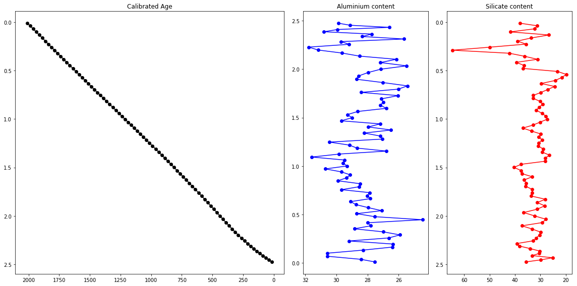
Does this help with the interpretation of the data?
fig = plt.figure(figsize=(16,8))


gs=GridSpec(2,4) # 2 rows, 4 columns

ax1=fig.add_subplot(gs[:,:2]) # Span all rows, firs two columns
ax2=fig.add_subplot(gs[:,2]) # Span all rows, third column
ax3=fig.add_subplot(gs[:,3]) # Span all rows, fourth column

ax1.set_title('Calibrated Age')
ax2.set_title('Aluminium content')
ax3.set_title('Silicate content')

ax1.plot(nframe_resampled['Age. Cal. CE'],nframe_resampled['depth (m)'],"k-o")
ax1.set_xlim(ax1.get_xlim()[::-1])
ax1.set_ylim(ax1.get_ylim()[::-1])

ax2.plot(nframe_resampled['Al'],nframe_resampled['depth (m)'],"b-o")
ax2.set_xlim(ax2.get_xlim()[::-1])
ax2.set_ylim(ax1.get_ylim()[::-1])

ax3.plot(nframe_resampled['Si'],nframe_resampled['depth (m)'],"r-o")
ax3.set_xlim(ax3.get_xlim()[::-1])
ax3.set_ylim(ax3.get_ylim()[::-1])

fig.tight_layout()
Numpy arrays to pandas dataframe
Write to csv file
import pathlib
import glob
import pandas as pd
import numpy as np
import os


path = '/opt/uio/deep_python/data/Nina/' #directory to the file we would like to import
filenames = glob.glob(path + "Inline_*.dat")

for file in filenames:
    print(file)
    data = np.loadtxt(file, dtype='str')
    frame=pd.DataFrame(data)
    frame[1].astype('float', inplace=True)
    frame[2].astype('float', inplace=True)
    frame[3] = frame[3].astype('float', inplace=True)+0.000001

    newfile = os.path.dirname(file) + '/' + pathlib.Path(file).stem + '_cal.dat'
    frame.to_csv(newfile, header=None, sep=' ', float_format="%.6f",  index=False)
/opt/uio/deep_python/data/Nina/Inline_3704.dat
/opt/uio/deep_python/data/Nina/Inline_3705.dat
/opt/uio/deep_python/data/Nina/Inline_3703.dat
/opt/uio/deep_python/data/Nina/Inline_3702.dat
/opt/uio/deep_python/data/Nina/Inline_3701.dat
Key Points