Visualize Climate data with Python
Overview
Teaching: 0 min
Exercises: 0 minQuestions
Learn to visualize Climate data?
Objectives
Learn to combine Climate data with your own research topic
Quick visualization
In this section, we will learn to read the metadata and visualize the NetCDF file we just downloaded.
Make sure you have installed Python along with the additional packages required to read Climate data files as described in the setup instructions.
The file we downloaded from CDS should be in your Downloads folder; to check it out, open a Terminal (Git bash terminal on windows) and type:
ls ~/Downloads/*.nc
For those of you who are not familiar with bash language:
the ~ symbol (a.k.a. tilde) is a shortcut for the home directory of a user;
*.nc means that we are looking for any files with a suffix .nc (NetCDF file).
adaptor.mars.internal-1559329510.4428957-10429-22-1005b553-e70d-4366-aa63-1424db2df740.nc
Then rename this file to a more friendly filename (please note that to ease further investigation, we add the date in the filename).
For instance, using bash:
mv ~/Downloads/adaptor.mars.internal-1559329510.4428957-10429-22-1005b553-e70d-4366-aa63-1424db2df740.nc ~/Downloads/ERA5_REANALYSIS_precipitation_200306.nc

ls ~/Downloads/*.nc
ERA5_REANALYSIS_precipitation_200306.nc
Start Anaconda Navigator, then select Environments:
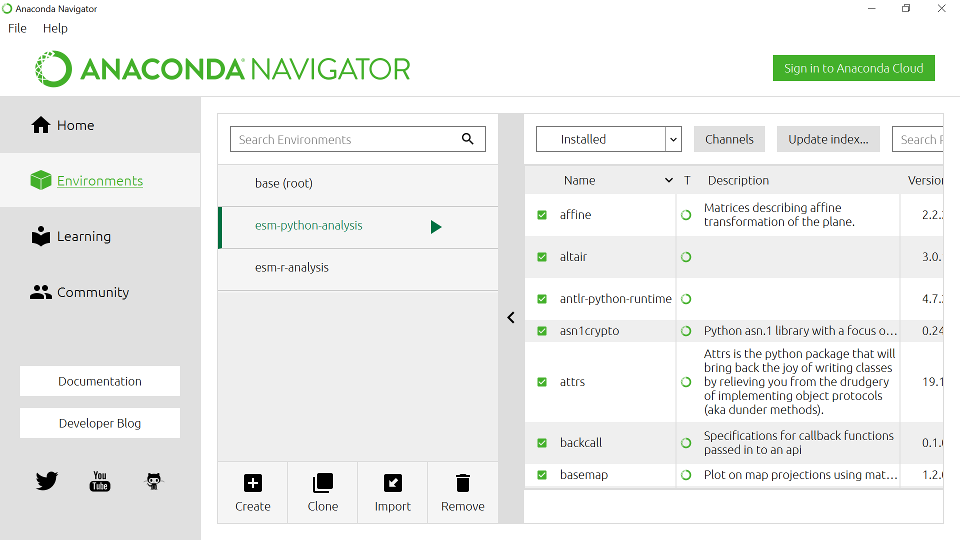
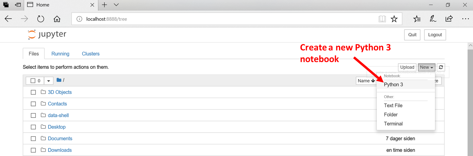
Select the esm-python-analysis environment and either left-click on the triangle/arrow next to it and Open with Jupyter Notebook, or go back to the Home tab and click on Launch to open your Jupyter Notebook :
Get metadata
import xarray as xr

# the line above is necessary for getting
# your plot embedded within the notebook
%matplotlib inline

dset = xr.open_dataset("~/Downloads/ERA5_REANALYSIS_precipitation_200306.nc")
print(dset)
Printing dset returns ERA5_REANALYSIS_precipitation_200306.nc metadata:
<xarray.Dataset>
Dimensions:    (latitude: 721, longitude: 1440, time: 1)
Coordinates:
  * longitude  (longitude) float32 0.0 0.25 0.5 0.75 ... 359.25 359.5 359.75
  * latitude   (latitude) float32 90.0 89.75 89.5 89.25 ... -89.5 -89.75 -90.0
  * time       (time) datetime64[ns] 2003-06-01
Data variables:
    tp         (time, latitude, longitude) float32 ...
Attributes:
    Conventions:  CF-1.6
    history:      2019-05-31 19:05:13 GMT by grib_to_netcdf-2.10.0: /opt/ecmw...
We can see that our dset object is an xarray.Dataset, which when printed shows all the metadata associated with our netCDF data file.
In this case, we are interested in the precipitation variable contained within that xarray Dataset:
print(dset['tp'])
<xarray.DataArray 'tp' (time: 1, latitude: 721, longitude: 1440)>
[1038240 values with dtype=float32]
Coordinates:
  * longitude  (longitude) float32 0.0 0.25 0.5 0.75 ... 359.25 359.5 359.75
  * latitude   (latitude) float32 90.0 89.75 89.5 89.25 ... -89.5 -89.75 -90.0
  * time       (time) datetime64[ns] 2003-06-01
Attributes:
    units:      m
    long_name:  Total precipitation
The total precipitation is in units of “metre of water per day”.
Quick visualization
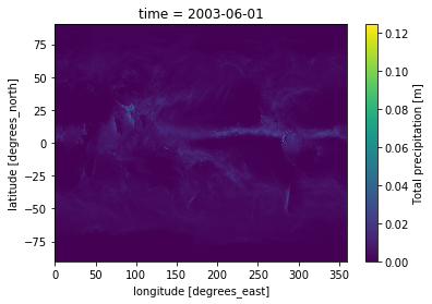
dset['tp'].plot()
We can change the colormap and adjust the maximum (remember the total precipitation is in metre):
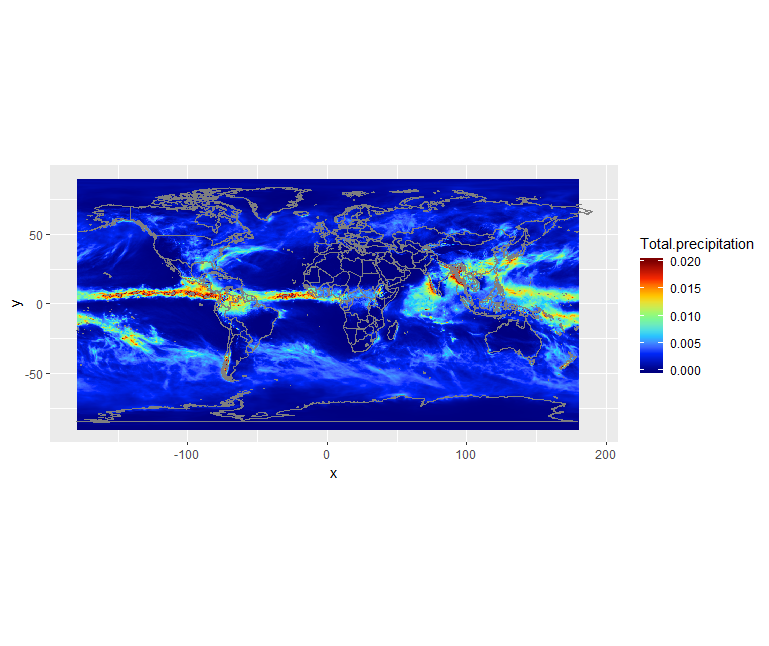
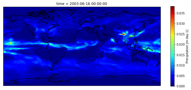
dset['tp'].plot(cmap='jet', vmax=0.02)
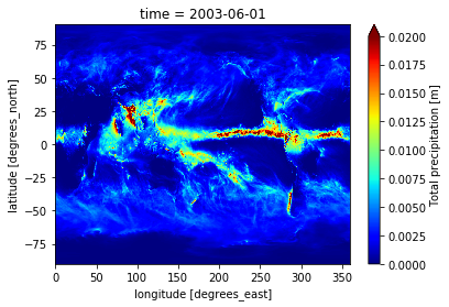
We can see there is a band around the equator and areas especially in Asia and South America with a lot of rain. Let’s add continents and a projection using cartopy:
import matplotlib.pyplot as plt
import cartopy.crs as ccrs

fig = plt.figure(figsize=[12,5])

# 111 means 1 row, 1 col and index 1
ax = fig.add_subplot(111, projection=ccrs.PlateCarree(central_longitude=0))

dset['tp'].plot(ax=ax, vmax=0.02, cmap='jet',
                   transform=ccrs.PlateCarree())
ax.coastlines()

plt.show()
At this stage, do not bother too much about the projection e.g. ccrs.PlateCarree.
We will discuss it in-depth in a follow-up episode.
Retrieve surface air temperature
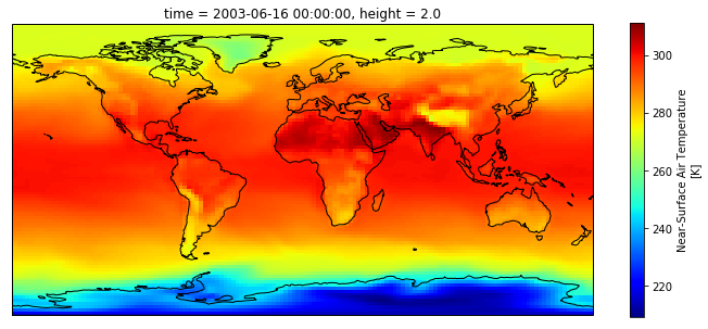
From the same product type (ERA5 single levels Monthly means) select 2m temperature. Make sure you rename your file to ERA5_REANALYSIS_air_temperature_200306.nc
- Inspect the metadata of the new retrieved file
- Visualize the 2m temperature with Python (using a similar script as for the total precipitation).
Solution with Python
dset = xr.open_dataset("~/Downloads/ERA5_REANALYSIS_air_temperature_200306.nc")
print(dset)

import matplotlib.pyplot as plt
import cartopy.crs as ccrs

fig = plt.figure(figsize=[12,5])

# 111 means 1 row, 1 col and index 1
ax = fig.add_subplot(111, projection=ccrs.PlateCarree(central_longitude=0))

dset['t2m'].plot(ax=ax,  cmap='jet',
                   transform=ccrs.PlateCarree())
ax.coastlines()

plt.show()
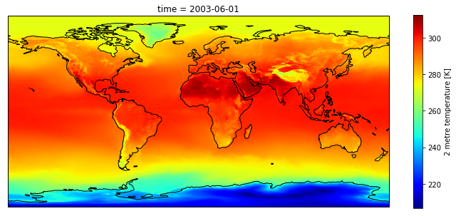
What is 2m temperature?
We selected ERA5 monthly averaged data on single levels from 1979 to present so we expected to get surface variables only. In fact, we get all the variables on a single level and usually close to the surface. Here 2m temperature is computed as the temperature at a reference height (2 metres). This corresponds to the surface air temperature.
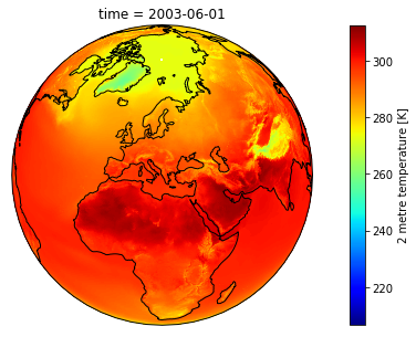
Change projection
It is very often convenient to visualize using a different projection than the original data:
import matplotlib.pyplot as plt
import cartopy.crs as ccrs

fig = plt.figure(figsize=[12,5])

# 111 means 1 row, 1 col and index 1
ax = fig.add_subplot(111, projection = ccrs.Orthographic(central_longitude=20, central_latitude=40))

dset['t2m'].plot(ax=ax,  cmap='jet',
                   transform=ccrs.PlateCarree())
ax.coastlines()

plt.show()
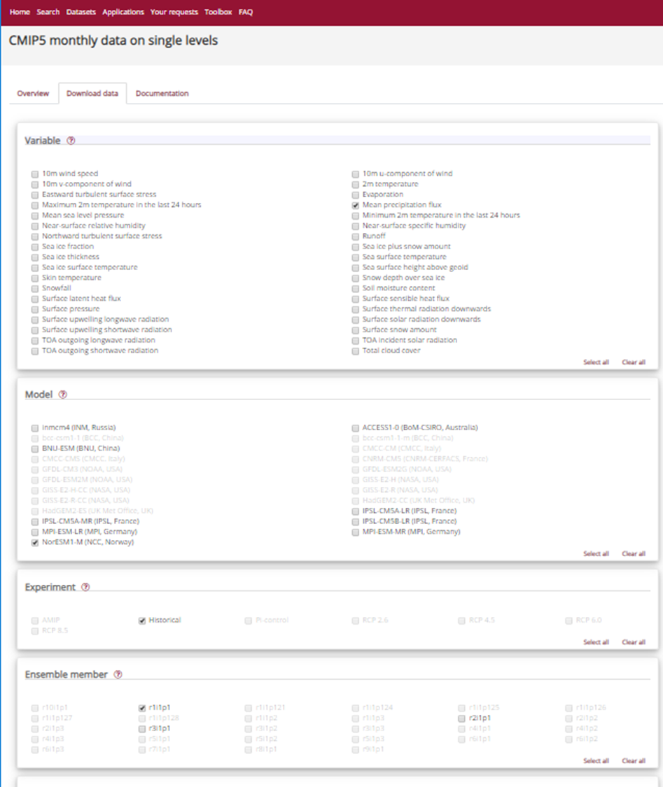
CMIP5 monthly data on single levels
Let’s have a look at CMIP 5 climate data.
Retrieve precipitation
We will retrieve precipitation from CMIP5 monthly data on single levels.
As you can see that you have the choice between several models, experiments and ensemble members.
CMIP5 models
CMIP5 (Coupled Model Intercomparison Project Phase 5) had the following objectives:
- evaluate how realistic the models are in simulating the recent past,
- provide projections of future climate change on two time scales, near term (out to about 2035) and long term (out to 2100 and beyond), and
- understand some of the factors responsible for differences in model projections, including quantifying some key feedbacks such as those involving clouds and the carbon cycle.
20 climate modeling groups from around the world participated to CMIP5. All the datasets are freely available from different repositories. For more information look here.
We will choose NorESM1-M (Norwegian Earth System Model 1 - medium resolution) based on the Norwegian Earth System Model.
Please note that it is very common to analyze several models instead of one to run statistical analysis.
CMIP5 Ensemble member
Many CMIP5 experiments, the so-called ensemble calculations, were calculated using several initial states, initialisation methods or physics details. Ensemble calculations facilitate quantifying the variability of simulation data concerning a single model.
In the CMIP5 project, ensemble members are named in the rip-nomenclature, r for realization, i for initialisation and p for physics, followed by an integer, e.g. r1i1p1. For more information look at Experiments, ensembles, variable names and other centralized properties.
Select:
- Model: NorESM1-M (NCC, Norway)
- Experiment: historical
- Ensemble: r1i1p1
- Period: 185001-200512
We rename the downloaded filename to pr_Amon_NorESM1-M_historical_r1i1p1_185001-200512.nc.
Let’s open this NetCDF file and check its metadata:
dset = xr.open_dataset("~/Downloads/pr_Amon_NorESM1-M_historical_r1i1p1_185001-200512.nc")
print(dset)
<xarray.Dataset>
Dimensions:    (bnds: 2, lat: 96, lon: 144, time: 1872)
Coordinates:
  * time       (time) object 1850-01-16 12:00:00 ... 2005-12-16 12:00:00
  * lat        (lat) float64 -90.0 -88.11 -86.21 -84.32 ... 86.21 88.11 90.0
  * lon        (lon) float64 0.0 2.5 5.0 7.5 10.0 ... 350.0 352.5 355.0 357.5
Dimensions without coordinates: bnds
Data variables:
    time_bnds  (time, bnds) object ...
    lat_bnds   (lat, bnds) float64 ...
    lon_bnds   (lon, bnds) float64 ...
    pr         (time, lat, lon) float32 ...
Attributes:
    institution:            Norwegian Climate Centre
    institute_id:           NCC
    experiment_id:          historical
    source:                 NorESM1-M 2011  atmosphere: CAM-Oslo (CAM4-Oslo-n...
    model_id:               NorESM1-M
    forcing:                GHG, SA, Oz, Sl, Vl, BC, OC
    parent_experiment_id:   piControl
    parent_experiment_rip:  r1i1p1
    branch_time:            255135.0
    contact:                Please send any requests or bug reports to noresm...
    initialization_method:  1
    physics_version:        1
    tracking_id:            5ccde64e-cfe8-47f6-9de8-9ea1621e7781
    product:                output
    experiment:             historical
    frequency:              mon
    creation_date:          2011-06-01T05:45:35Z
    history:                2011-06-01T05:45:35Z CMOR rewrote data to comply ...
    Conventions:            CF-1.4
    project_id:             CMIP5
    table_id:               Table Amon (27 April 2011) a5a1c518f52ae340313ba0...
    title:                  NorESM1-M model output prepared for CMIP5 historical
    parent_experiment:      pre-industrial control
    modeling_realm:         atmos
    realization:            1
    cmor_version:           2.6.0
This file contains monthly averaged data from January 1850 to December 2005. In CMIP the variable name for precipitation flux is called pr, so let’s look at the metadata:
print(dset.pr)
Note
The notation dset.pr is equivalent to dset[‘pr’].
<xarray.DataArray 'pr' (time: 1872, lat: 96, lon: 144)>
[25878528 values with dtype=float32]
Coordinates:
  * time     (time) object 1850-01-16 12:00:00 ... 2005-12-16 12:00:00
  * lat      (lat) float64 -90.0 -88.11 -86.21 -84.32 ... 84.32 86.21 88.11 90.0
  * lon      (lon) float64 0.0 2.5 5.0 7.5 10.0 ... 350.0 352.5 355.0 357.5
Attributes:
    standard_name:     precipitation_flux
    long_name:         Precipitation
    comment:           at surface; includes both liquid and solid phases from...
    units:             kg m-2 s-1
    original_name:     PRECT
    cell_methods:      time: mean
    cell_measures:     area: areacella
    history:           2011-06-01T05:45:35Z altered by CMOR: Converted type f...
    associated_files:  baseURL: http://cmip-pcmdi.llnl.gov/CMIP5/dataLocation...
The unit is: kg m-2 s-1. We want to convert the units from kg m-2 s-1 to something that we are a little more familiar with like mm day-1 or m day-1 (metre per day) that is what we had with ERA5.
To do this, consider that 1 kg of rain water spread over 1 m2 of surface is 1 mm in thickness and that there are 86400 seconds in one day. Therefore, 1 kg m-2 s-1 = 86400 mm day-1 or 86.4 m day-1.
So we can go ahead and multiply that array by 86.4 and update the units attribute accordingly:
dset.pr.data = dset.pr.data * 86.4
dset.pr.attrs['units'] = 'm/day'
Then we can select the data for June 2003 and plot the precipitation field:
import matplotlib.pyplot as plt
import cartopy.crs as ccrs

fig = plt.figure(figsize=[12,5])

# 111 means 1 row, 1 col and index 1
ax = fig.add_subplot(111, projection=ccrs.PlateCarree(central_longitude=0))

dset['pr'].sel(time='200306').plot(ax=ax, cmap='jet',
                   transform=ccrs.PlateCarree())
ax.coastlines()

plt.show()
To select June 2003, we used xarray select sel. This is a very powerful tool with which you can
specify a particular value you wish to select. You can also add a method such as nearest to select
the closest point to a given value. You can even select all the values inside a range (inclusive) with slice:
dset['pr'].sel(time=slice('200306', '200406', 12))
This command first takes the month of June 2003, then jumps 12 months and takes the month of June 2004.
<xarray.DataArray 'pr' (time: 2, lat: 96, lon: 144)>
array([[[2.114823e-05, 2.114823e-05, ..., 2.114823e-05, 2.114823e-05],
        [3.787203e-05, 3.682408e-05, ..., 3.772908e-05, 3.680853e-05],
        ...,
        [7.738324e-04, 8.255294e-04, ..., 7.871171e-04, 8.004216e-04],
        [6.984189e-04, 6.986369e-04, ..., 6.984310e-04, 6.983504e-04]],

       [[1.847185e-04, 1.847185e-04, ..., 1.847185e-04, 1.847185e-04],
        [8.476275e-05, 8.299961e-05, ..., 9.207508e-05, 8.666257e-05],
        ...,
        [4.763984e-04, 4.645830e-04, ..., 5.200990e-04, 4.929897e-04],
        [5.676933e-04, 5.677207e-04, ..., 5.673288e-04, 5.674717e-04]]],
      dtype=float32)
Coordinates:
  * time     (time) object 2003-06-16 00:00:00 2004-06-16 00:00:00
  * lat      (lat) float64 -90.0 -88.11 -86.21 -84.32 ... 84.32 86.21 88.11 90.0
  * lon      (lon) float64 0.0 2.5 5.0 7.5 10.0 ... 350.0 352.5 355.0 357.5
Attributes:
    standard_name:     precipitation_flux
    long_name:         Precipitation
    comment:           at surface; includes both liquid and solid phases from...
    units:             m day-1
    original_name:     PRECT
    cell_methods:      time: mean
    cell_measures:     area: areacella
    history:           2011-06-01T05:45:35Z altered by CMOR: Converted type f...
    associated_files:  baseURL: http://cmip-pcmdi.llnl.gov/CMIP5/dataLocation...
See here for more information.
Remark
We selected one year (2003) and one month (June) from both ERA5 and CMIP5 but only data from re-analysis (ERA5) corresponds to the actual month of June 2003. Data from the climate model (CMIP5 historical) is only “one realization” of a month of June, typical of present day conditions, but it cannot be considered as the actual weather at that date. To be more realistic, climate data has to be considered over a much longer period of time. For instance, we could easily compute (for both ERA5 and CMIP5) the average of the month of June between 1988 and 2018 (spanning 30 years) to have a more reliable results. However, as you (may) have noticed, the horizontal resolution of ERA5 (1/4 x 1/4 degrees) is much higher than that of the CMIP data (about 2 x 2 degrees) and therefore there is much more variability/details in the re-analysis data than with NorESM.
Plot surface air temperature with CMIP5 (June 2003)
When searching for CMIP5 monthly data on single levels you will see that you have the choice between several models and ensemble members. Select:
- Model: NorESM1-M (NCC, Norway)
- Ensemble: r1i1p1
Solution with Python
- Retrieve a new file with 2m temperature
- rename the retrieved file to tas_Amon_NorESM1-M_historical_r1i1p1_185001-200512.nc
dset = xr.open_dataset("~/Downloads/tas_Amon_NorESM1-M_historical_r1i1p1_185001-200512.nc")
print(dset)
<xarray.Dataset> Dimensions: (bnds: 2, lat: 96, lon: 144, time: 1872) Coordinates: * time (time) object 1850-01-16 12:00:00 ... 2005-12-16 12:00:00 * lat (lat) float64 -90.0 -88.11 -86.21 -84.32 ... 86.21 88.11 90.0 * lon (lon) float64 0.0 2.5 5.0 7.5 10.0 ... 350.0 352.5 355.0 357.5 height float64 ... Dimensions without coordinates: bnds Data variables: time_bnds (time, bnds) object ... lat_bnds (lat, bnds) float64 ... lon_bnds (lon, bnds) float64 ... tas (time, lat, lon) float32 ... Attributes: institution: Norwegian Climate Centre institute_id: NCC experiment_id: historical source: NorESM1-M 2011 atmosphere: CAM-Oslo (CAM4-Oslo-n... model_id: NorESM1-M forcing: GHG, SA, Oz, Sl, Vl, BC, OC parent_experiment_id: piControl parent_experiment_rip: r1i1p1 branch_time: 255135.0 contact: Please send any requests or bug reports to noresm... initialization_method: 1 physics_version: 1 tracking_id: c1dd6def-d613-43ab-a8b6-f4c80738f53b product: output experiment: historical frequency: mon creation_date: 2011-06-01T03:52:42Z history: 2011-06-01T03:52:42Z CMOR rewrote data to comply ... Conventions: CF-1.4 project_id: CMIP5 table_id: Table Amon (27 April 2011) a5a1c518f52ae340313ba0... title: NorESM1-M model output prepared for CMIP5 historical parent_experiment: pre-industrial control modeling_realm: atmos realization: 1 cmor_version: 2.6.0
- the name of the variable is tas (Near-Surface Air Temperature). We can print metadata for tas:
dset.tasYou can use dset[‘tas’] or dset.tas; the syntax is different but meaning is the same.
<xarray.DataArray 'tas' (time: 1872, lat: 96, lon: 144)>
[25878528 values with dtype=float32]
Coordinates:
 * time     (time) object 1850-01-16 12:00:00 ... 2005-12-16 12:00:00
 * lat      (lat) float64 -90.0 -88.11 -86.21 -84.32 ... 84.32 86.21 88.11 90.0
 * lon      (lon) float64 0.0 2.5 5.0 7.5 10.0 ... 350.0 352.5 355.0 357.5
   height   float64 ...
Attributes:
   standard_name:     air_temperature
   long_name:         Near-Surface Air Temperature
   units:             K
   original_name:     TREFHT
   cell_methods:      time: mean
   cell_measures:     area: areacella
   history:           2011-06-01T03:52:41Z altered by CMOR: Treated scalar d...
   associated_files:  baseURL: http://cmip-pcmdi.llnl.gov/CMIP5/dataLocation...
import matplotlib.pyplot as plt import cartopy.crs as ccrs fig = plt.figure(figsize=[12,5]) # 111 means 1 row, 1 col and index 1 ax = fig.add_subplot(111, projection=ccrs.PlateCarree(central_longitude=0)) dset['tas'].sel(time='200306').plot(ax=ax, cmap='jet', transform=ccrs.PlateCarree()) ax.coastlines() plt.show()
Retrieve Climate data with CDS API
Using CDS web interface is very useful when you need to retrieve small amount of data and you do not need to customize your request. However, it is often very useful to retrieve climate data directly on the computer where you need to run your postprocessing workflow.
In that case, you can use the CDS API (Application Programming Interface) to retrieve Climate data directly in Python from the Climate Data Store.
We will be using cdsapi python package.
Get your API key
-
Make sure you login to the Climate Data Store
-
Click on your username (top right of the main page) to get your API key.
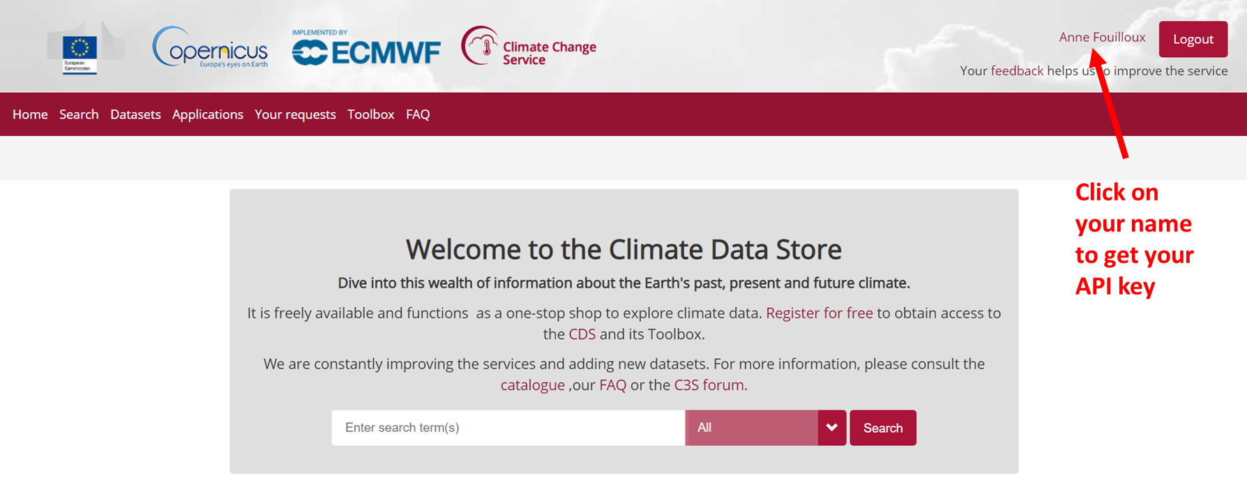
- Copy the code displayed beside, in the file
$HOME/.cdsapirc
url: https://cds.climate.copernicus.eu/api/v2
key: UID:KEY
Where UID is your uid and KEY your API key. See documentation
to get your API and related information.
Use CDS API
Once the CDS API client is installed, it can be used to request data from the datasets listed in the CDS catalogue. It is necessary to agree to the Terms of Use of every datasets that you intend to download.
Attached to each dataset download form, the button Show API Request displays the python code to be used. The request can be formatted using the interactive form. The api call must follow the syntax:
import cdsapi
c = cdsapi.Client()

c.retrieve("dataset-short-name",
           {... sub-selection request ...},
           "target-file")
For instance to retrieve the same ERA5 dataset e.g. near surface air temperature for June 2003:
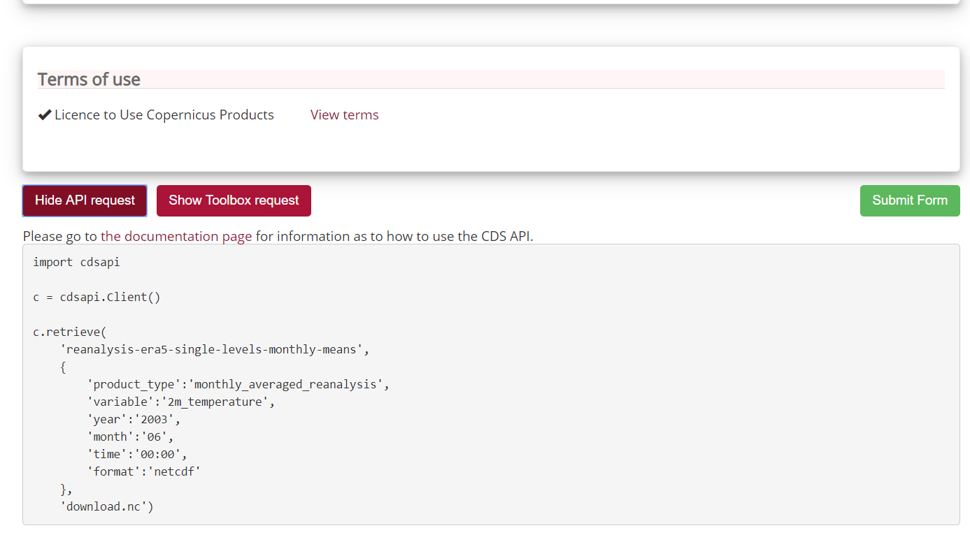
Let’s try it:
import cdsapi

c = cdsapi.Client()

c.retrieve(
    'reanalysis-era5-single-levels-monthly-means',
    {
        'product_type':'monthly_averaged_reanalysis',
        'variable':'2m_temperature',
        'year':'2003',
        'month':'06',
        'time':'00:00',
        'format':'netcdf'
    },
    'download.nc')
Geographical subset
import cdsapi

c = cdsapi.Client()

c.retrieve(
    'reanalysis-era5-single-levels-monthly-means',
    {
        'area'          : [60, -10, 50, 2], # North, West, South, East. Default: global
        'product_type':'monthly_averaged_reanalysis',
        'variable':'2m_temperature',
        'year':'2003',
        'month':'06',
        'time':'00:00',
        'format':'netcdf'
    },
    'download_small_area.nc')
Change horizontal resolution
For instance to get a coarser resolution:
import cdsapi

c = cdsapi.Client()

c.retrieve(
    'reanalysis-era5-single-levels-monthly-means',
    {
        'area'          : [60, -10, 50, 2], # North, West, South, East. Default: global
        'grid'          : [1.0, 1.0], # Latitude/longitude grid: east-west (longitude) and north-south resolution (latitude). Default: 0.25 x 0.25
        'product_type':'monthly_averaged_reanalysis',
        'variable':'2m_temperature',
        'year':'2003',
        'month':'06',
        'time':'00:00',
        'format':'netcdf'
    },
    'download_small.nc')
More information can be found here.
To download CMIP 5 Climate data via CDS API
import cdsapi

c = cdsapi.Client()

c.retrieve(
    'projections-cmip5-monthly-single-levels',
    {
        'variable':'2m_temperature',
        'model':'noresm1_m',
        'experiment':'historical',
        'ensemble_member':'r1i1p1',
        'period':'185001-200512'
    },
    'download_CMIP5.nc')
Download CMIP5 from Climate Data Store with
cdsapi
- Get near surface air temperature (2m temperature) and precipitation (mean precipitation flux) in one single request and save the result in a file
cmip5_sfc_monthly_1850-200512.zip- What do you get when you unzip this file?
Solution
- Download the file ~~~ import cdsapi
c = cdsapi.Client()
c.retrieve( ‘projections-cmip5-monthly-single-levels’, { ‘variable’:[ ‘2m_temperature’,’mean_precipitation_flux’ ], ‘model’:’noresm1_m’, ‘experiment’:’historical’, ‘ensemble_member’:’r1i1p1’, ‘period’:’185001-200512’, ‘format’:’tgz’ }, ‘cmip5_sfc_monthly_1850-200512.zip’)
{: .language-python}
- Uncompress it
If you select one variable, one experiment, one model, etc. then you get one file only and it is a netCDF file (even if it says otherwise!)
As soon as you select more than one variable, or more than one experiment, etc. then you get a zip or tgz (depending on the format you chose)
import os import zipfile
Create a new directory cmip5
os.mkdir(“./cmip5”)
zip_ref = zipfile.ZipFile(‘cmip5_sfc_monthly_1850-200512.zip’, ‘r’)
extract all the files in the new cmip5 directory
zip_ref.extractall(‘./cmip5’) zip_ref.close() ~~~
How to open several files with xarray?
In our last exercise, we downloaded two files, containing temperature and precipitation.
With xarray, it is possible to open these two files at the same time and get one unique view e.g.
very much like if we had one file only:
import xarray as xr

# use open_mfdataset to open alll netCDF files
# contained in the directory called cmip5
dset = xr.open_mfdataset("cmip5/*.nc")
print(dset)
    <xarray.Dataset>
    Dimensions:    (bnds: 2, lat: 96, lon: 144, time: 1872)
    Coordinates:
      * time       (time) object 1850-01-16 12:00:00 ... 2005-12-16 12:00:00
      * lat        (lat) float64 -90.0 -88.11 -86.21 -84.32 ... 86.21 88.11 90.0
      * lon        (lon) float64 0.0 2.5 5.0 7.5 10.0 ... 350.0 352.5 355.0 357.5
        height     float64 ...
    Dimensions without coordinates: bnds
    Data variables:
        time_bnds  (time, bnds) object dask.array<shape=(1872, 2), chunksize=(1872, 2)>
        lat_bnds   (lat, bnds) float64 dask.array<shape=(96, 2), chunksize=(96, 2)>
        lon_bnds   (lon, bnds) float64 dask.array<shape=(144, 2), chunksize=(144, 2)>
        pr         (time, lat, lon) float32 dask.array<shape=(1872, 96, 144), chunksize=(1872, 96, 144)>
        tas        (time, lat, lon) float32 dask.array<shape=(1872, 96, 144), chunksize=(1872, 96, 144)>
    Attributes:
        institution:            Norwegian Climate Centre
        institute_id:           NCC
        experiment_id:          historical
        source:                 NorESM1-M 2011  atmosphere: CAM-Oslo (CAM4-Oslo-n...
        model_id:               NorESM1-M
        forcing:                GHG, SA, Oz, Sl, Vl, BC, OC
        parent_experiment_id:   piControl
        parent_experiment_rip:  r1i1p1
        branch_time:            255135.0
        contact:                Please send any requests or bug reports to noresm...
        initialization_method:  1
        physics_version:        1
        tracking_id:            5ccde64e-cfe8-47f6-9de8-9ea1621e7781
        product:                output
        experiment:             historical
        frequency:              mon
        creation_date:          2011-06-01T05:45:35Z
        history:                2011-06-01T05:45:35Z CMOR rewrote data to comply ...
        Conventions:            CF-1.4
        project_id:             CMIP5
        table_id:               Table Amon (27 April 2011) a5a1c518f52ae340313ba0...
        title:                  NorESM1-M model output prepared for CMIP5 historical
        parent_experiment:      pre-industrial control
        modeling_realm:         atmos
        realization:            1
        cmor_version:           2.6.0
How to use xarray to get metadata?
Get the list of variables
for varname, variable in dset.items():
    print(varname)
    time_bnds
    lat_bnds
    lon_bnds
    pr
    tas
Create a python dictionary with variable and long name
dict_variables = {}
for varname, variable in dset.items():
    if len(dset[varname].attrs) > 0:
        dict_variables[dset[varname].attrs['long_name']] = varname
print(dict_variables)
print(list(dict_variables.keys()))
    {'Precipitation': 'pr', 'Near-Surface Air Temperature': 'tas'}
    ['Precipitation', 'Near-Surface Air Temperature']
Select temperature (tas)
- two notations for accessing variables
dset.tas
    <xarray.DataArray 'tas' (time: 1872, lat: 96, lon: 144)>
    dask.array<shape=(1872, 96, 144), dtype=float32, chunksize=(1872, 96, 144)>
    Coordinates:
      * time     (time) object 1850-01-16 12:00:00 ... 2005-12-16 12:00:00
      * lat      (lat) float64 -90.0 -88.11 -86.21 -84.32 ... 84.32 86.21 88.11 90.0
      * lon      (lon) float64 0.0 2.5 5.0 7.5 10.0 ... 350.0 352.5 355.0 357.5
        height   float64 ...
    Attributes:
        standard_name:     air_temperature
        long_name:         Near-Surface Air Temperature
        units:             K
        original_name:     TREFHT
        cell_methods:      time: mean
        cell_measures:     area: areacella
        history:           2011-06-01T03:52:41Z altered by CMOR: Treated scalar d...
        associated_files:  baseURL: http://cmip-pcmdi.llnl.gov/CMIP5/dataLocation...
dset['tas']
    <xarray.DataArray 'tas' (time: 1872, lat: 96, lon: 144)>
    dask.array<shape=(1872, 96, 144), dtype=float32, chunksize=(1872, 96, 144)>
    Coordinates:
      * time     (time) object 1850-01-16 12:00:00 ... 2005-12-16 12:00:00
      * lat      (lat) float64 -90.0 -88.11 -86.21 -84.32 ... 84.32 86.21 88.11 90.0
      * lon      (lon) float64 0.0 2.5 5.0 7.5 10.0 ... 350.0 352.5 355.0 357.5
        height   float64 ...
    Attributes:
        standard_name:     air_temperature
        long_name:         Near-Surface Air Temperature
        units:             K
        original_name:     TREFHT
        cell_methods:      time: mean
        cell_measures:     area: areacella
        history:           2011-06-01T03:52:41Z altered by CMOR: Treated scalar d...
        associated_files:  baseURL: http://cmip-pcmdi.llnl.gov/CMIP5/dataLocation...
Get attributes
dset['tas'].attrs['long_name']
'Near-Surface Air Temperature'
dset['tas'].attrs['units']
'K'
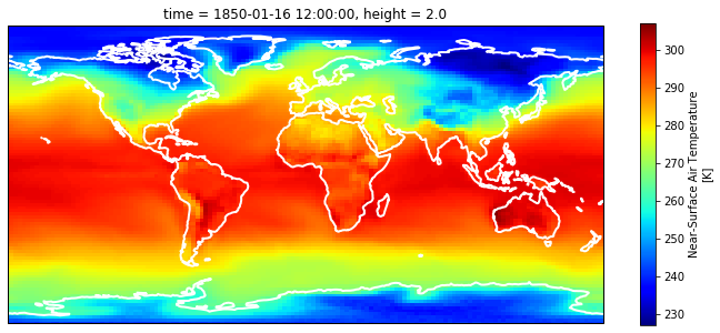
How to create a function to generate a plot for a given date and given variable?
Instead of copy-paste the same code several times to plot different variables and dates, it is common to define a function with the date and variable as parameters:
import matplotlib.pyplot as plt
import cartopy.crs as ccrs

def generate_plot(date, variable):

    fig = plt.figure(figsize=[12,5])

    # 111 means 1 row, 1 col and index 1
    ax = fig.add_subplot(111, projection=ccrs.PlateCarree(central_longitude=0))

    dset[variable].sel(time=date).plot(cmap='jet',
                                      transform=ccrs.PlateCarree())
    ax.coastlines(color='white', linewidth=2.)
Call generate_plot function to plot 2m temperature
generate_plot(dset.time.values.tolist()[0], 'tas')
Plotting on-demand with Jupyter widgets
Our goal in this section is to learn to create a user interface where one can select the variable and date to plot.
Create a widget to select available variables
%matplotlib inline
import ipywidgets as widgets
select_variable = widgets.Select(
    options=['2m temperature', 'precipitation'],
    value='2m temperature',
    rows=2,
    description='Variable:',
    disabled=False
)

display(select_variable)
{. .language-python}
Create a widget to select date (year and month)
%matplotlib inline
import ipywidgets as widgets
select_date = widgets.Dropdown(
    options=dset.time.values.tolist(),
    rows=2,
    description='Date:',
    disabled=False
)

display(select_date)
Use widgets to plot the chosen variable at the chosen date
import ipywidgets as widgets
import matplotlib.pyplot as plt
import cartopy.crs as ccrs

# widget for variables
list_variables = list(dict_variables.keys())
select_variable = widgets.Select(
    options=list_variables,
    value=list_variables[0],
    rows=2,
    description='Variable:',
    disabled=False
)

# Widget for date
select_date = widgets.Dropdown(
    options=dset.time.values.tolist(),
    rows=2,
    description='Date:',
    disabled=False
)

# generate plot
def generate_plot(date, variable):

    fig = plt.figure(figsize=[12,5])

    # 111 means 1 row, 1 col and index 1
    ax = fig.add_subplot(111, projection=ccrs.PlateCarree(central_longitude=0))

    dset[dict_variables[variable]].sel(time=date).plot(cmap='jet',
                                      transform=ccrs.PlateCarree())
    ax.coastlines(color='white', linewidth=2.)


interact_plot = widgets.interact(generate_plot, date = select_date, variable = select_variable);
Remark
The plot does not change in the image above because we only have static HTML pages. However, you can test it with mybinder:
.
Key Points
xarray
cartopy
CDS API for Python