Cloud feedback Analysis with ERA5 high-resolution (~0.25deg) monthly means
Contents
Cloud feedback Analysis with ERA5 high-resolution (~0.25deg) monthly means
Table of Contents
1. Introduction 
Cloud feedbacks are a major contributor to the spread of climate sensitivity in global climate models (GCMs) (Zelinka et al. (2020)]). Among the most poorly understood cloud feedbacks is the one associated with the cloud phase, which is expected to be modified with climate change (Bjordal et al. (2020)). Cloud phase bias, in addition, has significant implications for the simulation of radiative properties and glacier and ice sheet mass balances in climate models.
In this context, this work aims to expand our knowledge on how the representation of the cloud phase affects snow formation in GCMs. Better understanding this aspect is necessary to develop climate models further and improve future climate predictions.
Load ERA5 data previously downloaded locally via Jupyter Notebook - download ERA5
find clouds: liquid-only, ice-only, mixed-phase
Regridd the ERA5 variables to the same horizontal resolution as high-resolution CMIP6 models with
xesmfCalculate and plot the seasonal mean of the variable
Questions
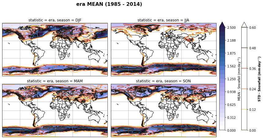
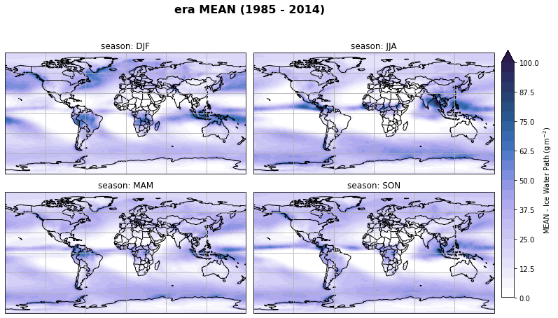
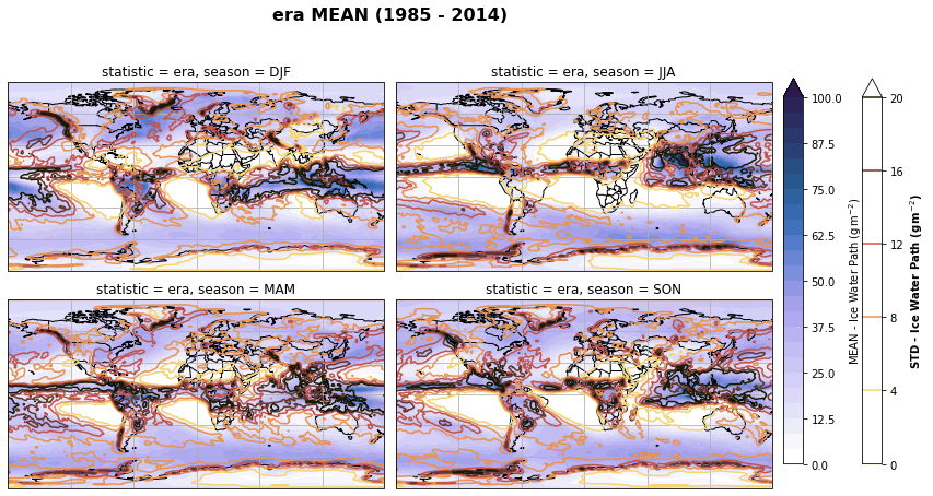
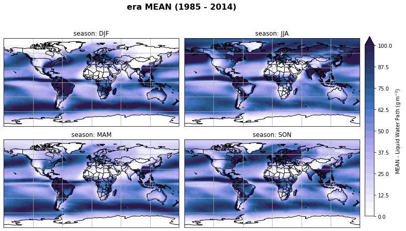
How is the cloud phase and snowfall varying between 1985 and 2014?
NOTE: We answer questions related to the comparison of CMIP models to ERA5 in another Jupyter Notebook.
2. Data Wrangling 
This study will compare surface snowfall, ice, and liquid water content from the Coupled Model Intercomparison Project Phase 6 (CMIP6) climate models (accessed through Pangeo) to the European Centre for Medium-Range Weather Forecast Re-Analysis 5 (ERA5) data from 1985 to 2014. We conduct statistical analysis at the annual and seasonal timescales to determine the biases in cloud phase and precipitation (liquid and solid) in the CMIP6 models and their potential connection between them. The CMIP6 data analysis can be found in the Jupyter Notebook for CMIP6.
Time period: 1985 to 2014
horizonal resolution: ~0.25deg
time resolution: monthly atmospheric data
Variables:
shortname |
Long name |
Units |
levels |
|---|---|---|---|
sf |
snowfall |
[m of water eq] |
surface |
msr |
mean_snowfall_rate |
[kg m-2 s-1] |
surface |
cswc |
specific_snow_water_content |
[kg kg-1] |
pl |
clwc |
specific_cloud_liquid_water_content |
[kg kg-1] |
pl |
clic |
specific_cloud_ice_water_content |
[kg kg-1] |
pl |
t |
temperature |
[K] |
pl |
2t |
2 metre temperature |
[K] |
surface |
tclw |
Total column cloud liquid water |
[kg m-2] |
single |
tciw |
Total column cloud ice water |
[kg m-2] |
single |
tp |
Total precipitation |
[m] |
surface |
Import python packages
Pythonenvironment requirements: file globalsnow.ymlload
pythonpackages from imports.pyload
functionsfrom functions.py
# supress warnings
import warnings
warnings.filterwarnings('ignore') # don't output warnings

# import packages
import sys
import os
if os.path.isfile('/uio/kant/geo-metos-u1/franzihe/Documents/Python/globalsnow/eosc-nordic-climate-demonstrator/work/utils/imports.py') == True:
    sys.path.append('/uio/kant/geo-metos-u1/franzihe/Documents/Python/globalsnow/eosc-nordic-climate-demonstrator/work/utils')

elif os.path.isfile('/uio/kant/geo-metos-u1/franzihe/Documents/Python/globalsnow/eosc-nordic-climate-demonstrator/work/utils/imports.py') == False:
    sys.path.append('/home/franzihe/Documents/Python/eosc-nordic-climate-demonstrator/work/utils/')

from imports import(xr, intake, ccrs, cy, plt, glob, cm, fct, np, da)
xr.set_options(display_style='html')
<xarray.core.options.set_options at 0x7f60fbc9d100>
# reload imports
%load_ext autoreload
%autoreload 2
Open ERA5 variables
Get the data requried for the analysis. Beforehand we downloaded the monthly averaged data on single levels and pressure levels via the Climate Data Store (CDS) infrastructure. The github repository Download ERA5 gives examples on how to download the data from the CDS. We use the Jupyter Notebooks download_Amon_single_level and download_Amon_pressure_level. Both, download the monthly means for the variables mentioned above between 1985 and 2014.
NOTE: To download from CDS a user has to have a CDS user account, please create the account here.
The ERA5 0.25deg data is located in the folder /input/ERA5/monthly_means/0.25deg.
if (len(glob('/scratch/franzihe/input/ERA5/monthly_means/0.25deg/*_Amon_ERA5_*12.nc')) > 0) == True:
    input_data = '/scratch/franzihe/input'
    output_data = '/scratch/franzihe/output'

if (len(glob('/home/franzihe/Data/input/ERA5/monthly_means/0.25deg/*_Amon_ERA5_*12.nc')) > 0) == True:
    input_data = '/home/franzihe/Data/input/'
    output_data = '/home/franzihe/Data/output'
era_in = '{}/ERA5/monthly_means/0.25deg'.format(input_data)
era_out = '{}/ERA5/monthly_means/1deg'.format(output_data)
variable_id=[
            '2t',
            'clic',
            'clwc',
            'cswc',
            'msr',
            'sf',
            't',
            'tciw',
            'tclw',
            'tp'
             ]
At the moment we have downloaded 30 years (1985-2014) for ERA5. We define start and end year to ensure to only extract the 30-year period between 1985 and 2014.
\(\rightarrow\) Define a start and end year
We will load all available variables into one xarray dataset with xarray.open_mfdataset(file) and select the time range by name.
starty = 1985; endy = 2014
year_range = range(starty, endy+1)
# Input data from ERA5 with a resolution of 0.25x0.25deg to be regridded
era_file_in = glob('{}/*_Amon_ERA5_*12.nc'.format(era_in, ))       # search for data in the local directory
ds_era = xr.open_mfdataset(era_file_in)
ds_era = ds_era.sel(time = ds_era.time.dt.year.isin(year_range)).squeeze()
# create pressure array
ds_era['pressure'] = xr.DataArray(data=da.ones(shape = ds_era['clwc'].shape, chunks=(ds_era['clwc'].shape[0]/3, ds_era['clwc'].shape[1], ds_era['clwc'].shape[2], ds_era['clwc'].shape[3]/2)),
                                                               dims=list(ds_era['clwc'].dims),
                                                               coords=[ds_era.time.values, ds_era.level.values, ds_era.latitude.values, ds_era.longitude.values])

ds_era['pressure'] = ds_era['pressure']*ds_era['level'][::-1]
Change attributes matching CMIP6 data
We will assign the attributes to the variables to make CMIP6 and ERA5 variables comperable.
The data documentation of monthly means gives information about the accumulations in monthly means (of daily means, stream=moda/edmo). Hence, the precipitation variables have been scaled to have an “effective” processing period of one day, so for accumulations in these streams
sfis in m of water per day \(\rightarrow\) multiply by 1000 to get kg m-2 day-1 or mmday-1.tpis in m \(\rightarrow\) Multiply by 1000 to get mmciwc,clwc, andcswcis in kg kg-1 \(\rightarrow\) Multiply by 1000 to get g kg-1msris in kg m-2 s-1 \(\rightarrow\) Multiply by 86400 to get mm day-1tciwandtclwis in kg m-2 \(\rightarrow\) Multiply by 1000 to get g m-2
# rename variable name to variable id
# variable_id[variable_id.index('2t')] = 't2m'
variable_id[variable_id.index('clic')] = 'ciwc'

# rename variable name in dataset to match variable_id
ds_era = ds_era.rename({'t2m':'2t'})
for var_id in variable_id:

    if var_id == 'ciwc' or var_id == 'clwc' or var_id == 'cswc' or var_id == 'sf' or var_id == 'tciw' or var_id == 'tclw' or var_id == 'tp':
        ds_era[var_id] = ds_era[var_id]*1000

        if var_id == 'ciwc':
            ds_era[var_id].attrs = {'units': 'g kg-1', 'long_name':'Specific cloud ice water content'}
        if var_id == 'clwc':
            ds_era[var_id].attrs = {'units': 'g kg-1', 'long_name':'Specific cloud liquid water content'}
        if var_id == 'cswc':
            ds_era[var_id].attrs = {'units': 'g kg-1', 'long_name':'Specific snow water content'}
        if var_id == 'sf':
            ds_era[var_id].attrs = {'units': 'mm day-1', 'long_name': 'Snowfall',}
        if var_id == 'tciw':
            ds_era[var_id].attrs = {'units': 'g m-2', 'long_name': 'Total column cloud ice water'}
        if var_id == 'tclw':
            ds_era[var_id].attrs = {'units': 'g m-2', 'long_name': 'Total column cloud liquid water'}
        if var_id == 'tp':
            ds_era[var_id].attrs = {'units': 'mm', 'long_name': 'Total precipitation'}

    if var_id == 'msr':
        ds_era[var_id] = ds_era[var_id]*86400
        ds_era[var_id].attrs = {'units': 'mm day-1', 'long_name': 'Mean snowfall rate'}
Find mixed-phase clouds
Calculate the IWC/LWC statistics given by the values. Setting the value to 0.5 will find the level in the atmosphere where IWC and LWC are 50/50. Setting it to a value of 0.7 will find the level where IWC is 70% while LWC is 30%.
find the fraction of IWC to LWC $\(fraction = \frac{IWC}{IWC + LWC}\)$
find the nearest value to given IWC-fraction
find atmospheric pressure levels where IWC/LWC fraction occurs
find the index of the first atmospheric pressure level
use the index to select variables
# create occcurence array
for var_id in list(ds_era.keys()):
    ds_era[var_id + '_occurence'] = xr.DataArray(data=da.ones(shape = (ds_era['time'].shape[0],ds_era['latitude'].shape[0], ds_era['longitude'].shape[0]), chunks=(ds_era['time'].shape[0]/3, ds_era['latitude'].shape[0], ds_era['longitude'].shape[0]/2)),
                                                                dims=[ds_era['time'].dims[0],ds_era['latitude'].dims[0], ds_era['longitude'].dims[0]] ,
                                                                coords=[ds_era['time'].values,ds_era['latitude'].values, ds_era['longitude'].values] )
Create dictionary from the list of datasets we want to use for the IWC/LWC statistics
iwc_stat = {'50':0.5, '70':0.7, '30':0.5}

dset_dict = dict()
dset_dict['era'] = ds_era
for i in iwc_stat.items():
    dset_dict['era_{}'.format(i[0])] = fct.find_IWC_LWC_level(ds_era, var1='ciwc', var2='clwc', value=i[1], coordinate='level')

    # rename latitude and longitude
    dset_dict['era_{}'.format(i[0])] = fct.rename_coords_lon_lat(dset_dict['era_{}'.format(i[0])])
Regrid ERA5 data to common NorESM2-MM grid 
We want to conduct statistical analysis at the annual and seasonal timescales to determine the biases in cloud phase and precipitation (liquid and solid) for the CMIP6 models in comparison to ERA5.
The ERA5 data has a nominal resolution of 0.25 deg and has to be regridded to the same horizontal resolution as the NorESM2-MM. Hence we will make use of the python package xesmf and decreasing resolution, Limitations and warnings.
\(\rightarrow\) Define NorESM2-MM as the reference grid ds_out.
Save all variables in one file and each variable to a netcdf datasets between 1985 an 2014, locally.
NOTE: This can take a while, so be patient
# Read in the output grid from NorESM
cmip_file = '/scratch/franzihe/input/cmip6_hist/1deg/grid_NorESM2-MM.nc'
ds_out = xr.open_dataset(cmip_file)


# create dictionary for reggridded data
ds_gridded_dict = dict()

counter = 0

for keys in dset_dict.keys():

    # select where data should be saved
    filename = '{}_Amon_1deg_{}01_{}12.nc'.format(keys,starty, endy)
    era_file_out = era_out + '/Amon/' + filename
    files = glob(era_file_out)


    # Regrid data
    ds_in_regrid = fct.regrid_data(dset_dict[keys], ds_out)

    # Shift the longitude from 0-->360 to -180-->180 and sort by longitude and time
    ds_in_regrid = ds_in_regrid.assign_coords(lon=(((ds_in_regrid.lon + 180) % 360) - 180)).sortby('lon').sortby('time')

    # create dataset with all statistics
    ds_gridded_dict[keys] = ds_in_regrid

    # if era_file_out in files:
    #     print('{} is downloaded'.format(era_file_out))
    #     counter += 1
    #     print('Have regridded in total: {:} files'.format(str(counter)))
    # else: # Save to netcdf file
    ds_in_regrid.to_netcdf(era_file_out)
    print('file written: {}'.format(era_file_out))
The following cell is not needed
Fix the regridding for the ERA5 data.
ds_gridded_dict = dict()
ds_gridded_dict['era'] = xr.open_dataset('/scratch/franzihe/output/ERA5/monthly_means/1deg/Amon/all_Amon_1deg_198501_201412.nc')

# rename temperature variable
ds_gridded_dict['era'] = ds_gridded_dict['era'].rename({'t2m':'2t'})


# create pressure array
ds_gridded_dict['era']['pressure'] = xr.DataArray(data=da.ones(shape = ds_gridded_dict['era']['clwc'].shape, chunks=(120, 37, 721, 1440/2)
),
                                                               dims=list(ds_gridded_dict['era']['clwc'].dims),
                                                               coords=[ds_gridded_dict['era'].time.values, ds_gridded_dict['era'].level.values, ds_gridded_dict['era'].lat.values, ds_gridded_dict['era'].lon.values])

ds_gridded_dict['era']['pressure'] = ds_gridded_dict['era']['pressure']*ds_gridded_dict['era']['level'][::-1]

# create occcurence array
for var_id in list(ds_gridded_dict['era'].keys()):
    ds_gridded_dict['era'][var_id + '_occurence'] = xr.DataArray(data=da.ones(shape = (ds_gridded_dict['era']['time'].shape[0],ds_gridded_dict['era']['lat'].shape[0], ds_gridded_dict['era']['lon'].shape[0]), chunks=(ds_gridded_dict['era']['time'].shape[0]/3, ds_gridded_dict['era']['lat'].shape[0], ds_gridded_dict['era']['lon'].shape[0]/2)),
                                                                dims=[ds_gridded_dict['era']['time'].dims[0],ds_gridded_dict['era']['lat'].dims[0], ds_gridded_dict['era']['lon'].dims[0]] ,
                                                                coords=[ds_gridded_dict['era']['time'].values,ds_gridded_dict['era']['lat'].values, ds_gridded_dict['era']['lon'].values] )


for i in iwc_stat.items():
    ds_gridded_dict['era_{}'.format(i[0])] = fct.find_IWC_LWC_level(ds_gridded_dict['era'], var1 ='ciwc', var2='clwc', value=i[1], coordinate='level')
Connect all statistics into one Dataset with new coordinate ‘statistic’
We will create a xarray.Dataset with all ERA5 data, after the interpolation to the same horizonal (and vertical) resolution. This step will make the next steps easier, as we will not need the the full dictonary key and can just use the names.
_ds = list(dset_dict.values())
_coord = list(dset_dict.keys())
ds_era_025deg = xr.concat(objs=_ds, dim=_coord, coords="all").rename({'concat_dim':'statistic'})
_ds = list(ds_gridded_dict.values())
_coord = list(ds_gridded_dict.keys())
ds_era_1deg = xr.concat(objs=_ds, dim=_coord, coords="all").rename({'concat_dim':'statistic'})
3. Exploratory Data Analysis 
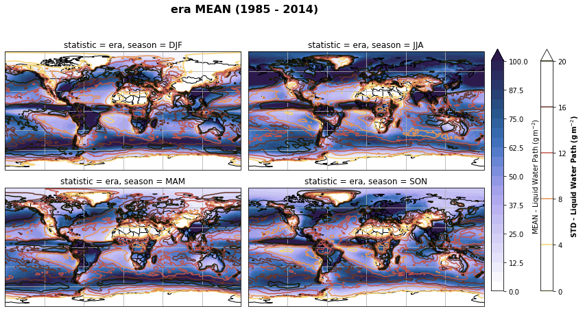
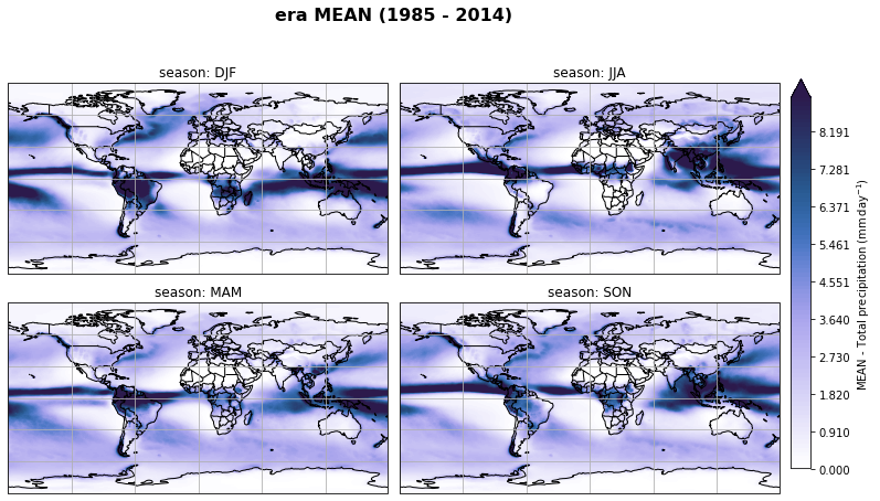
Create seasonal mean/spread of all ERA5 data
…and plot seasonal mean of each individual, like ERA5-0.25deg resolution, ERA5-1deg resolution, and the IWC/LWC statistics for 50%, 70%, 30% respectively.
# Create seasonal mean of variables
for var_id in list(ds_era_1deg.keys()):
    ds_era_1deg = fct.seasonal_mean_std(ds_era_1deg, var_id)

for var_id in list(ds_era_025deg.keys()):
    ds_era_025deg = fct.seasonal_mean_std(ds_era_025deg, var_id)
stat = 'era'
for var_id in variable_id:
if var_id == 'msr':
continue
else:
# for stat in ds_era_1deg.statistic.values:
if len(ds_era_1deg[var_id].sel(statistic=stat).dims) <= 3:
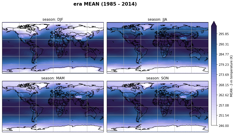
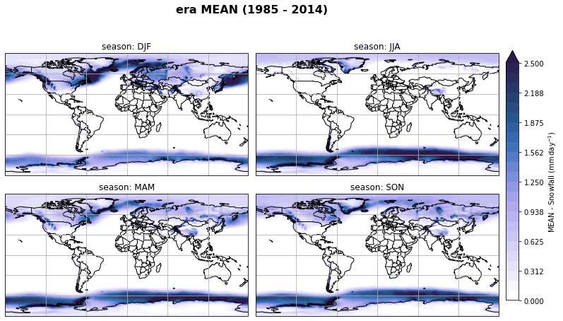
# Plot seasonal mean
fig, axs, im = fct.plt_spatial_seasonal_mean(ds_era_1deg[var_id+'_season_mean'].sel(statistic=stat), var_id, add_colorbar=False, title='{} MEAN ({} - {})'.format(stat, starty, endy))
fig.subplots_adjust(right=0.8)
cbar_ax = fig.add_axes([1, 0.15, 0.025, 0.7])
cb = fig.colorbar(im, cax=cbar_ax, orientation="vertical", fraction=0.046, pad=0.04)
cb.set_label(label='MEAN - {}'.format(fct.plt_dict[var_id][fct.plt_dict['header'].index('label')], weight='bold'))
plt.tight_layout()
# save figure to png
figdir = '/uio/kant/geo-metos-u1/franzihe/Documents/Figures/ERA5/'
figname = '{}_{}_season_1deg_{}_{}.png'.format(var_id,stat, starty, endy)
plt.savefig(figdir + figname, format = 'png', bbox_inches = 'tight', transparent = False)
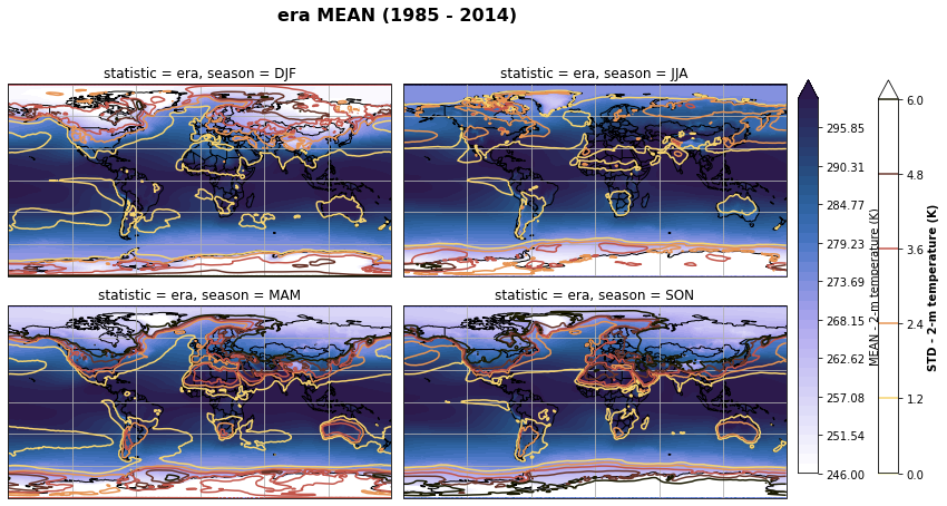
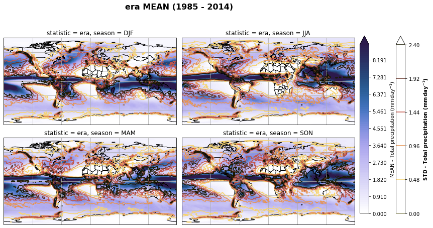
# Plot seasonal mean and std
fig, axs, im = fct.plt_spatial_seasonal_mean(ds_era_1deg[var_id+'_season_mean'].sel(statistic=stat), var_id, add_colorbar=False, title='{} MEAN ({} - {})'.format(stat, starty, endy))
fig.subplots_adjust(right=0.8)
cbar_ax = fig.add_axes([1, 0.15, 0.025, 0.7])
cb = fig.colorbar(im, cax=cbar_ax, orientation="vertical", fraction=0.046, pad=0.04)
cb.set_label(label='MEAN - {}'.format(fct.plt_dict[var_id][fct.plt_dict['header'].index('label')], weight='bold'))
for ax, i in zip(axs, ds_era_1deg[var_id+'_season_std'].sel(statistic=stat).season):
sm = ds_era_1deg[var_id+'_season_std'].sel(season=i, statistic=stat).plot.contour(ax=ax, transform=ccrs.PlateCarree(),
robust=True,
vmin = fct.plt_dict[var_id][fct.plt_dict['header'].index('vmin_std')],
vmax = fct.plt_dict[var_id][fct.plt_dict['header'].index('vmax_std')],
levels = 6,
cmap=cm.lajolla,
add_colorbar=False)
cbar_ax = fig.add_axes([1.10, 0.15, 0.025, 0.7])
sb = fig.colorbar(sm, cax=cbar_ax, orientation="vertical", fraction=0.046, pad=0.04)
sb.set_label(label='STD - {}'.format(fct.plt_dict[var_id][fct.plt_dict['header'].index('label')]), weight='bold')
plt.tight_layout()
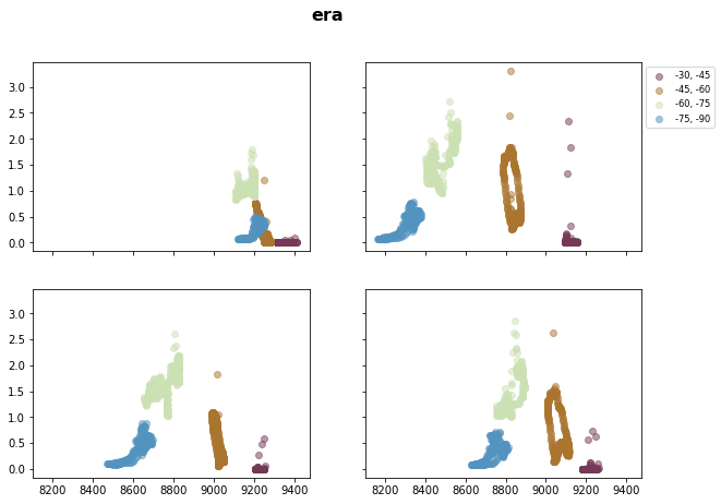
Calculate latitude band mean of variables
We will only use high latitudes and the extratropics the latitude bands are as follow:
Southern Hemispher:
[-30, -45)
[-45, -60)
[-60, -75)
[-75, -90)
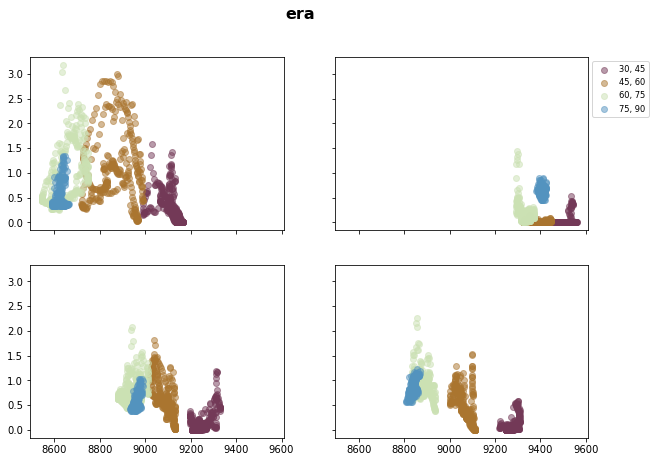
Northern Hemisphere:
[30, 45)
[45, 60)
[60, 75)
[75, 90)
lat_SH = (-90, -30); lat_NH = (30,90); step = 15
iteration_SH = range(lat_SH[1], lat_SH[0], -step)
iteration_NH = range(lat_NH[0], lat_NH[1], step)
for var_id in ds_era.keys():
    for _lat in iteration_SH:

        # ERA5 original resolution
        ds_era_025deg[var_id + '_season_{}_{}'.format(_lat, _lat-step)] = ds_era_025deg[var_id + '_season_mean'].sel(lat = slice(_lat, _lat-step)).mean(('lat',), keep_attrs=True, skipna=True)

        # ERA5 regridded resolution
        ds_era_1deg[var_id + '_season_{}_{}'.format(_lat, _lat-step)] = ds_era_1deg[var_id + '_season_mean'].sel(lat = slice(_lat-step, _lat)).mean(('lat',), keep_attrs=True, skipna=True)

    for _lat in iteration_NH:
        # ERA5 original resolution
        ds_era_025deg[var_id + '_season_{}_{}'.format(_lat, _lat+step)] = ds_era_025deg[var_id + '_season_mean'].sel(lat = slice(_lat+step, _lat)).mean(('lat',), keep_attrs=True, skipna=True)

        # ERA5 regridded resolution
        ds_era_1deg[var_id + '_season_{}_{}'.format(_lat, _lat+step)] = ds_era_1deg[var_id + '_season_mean'].sel(lat = slice(_lat, _lat+step)).mean(('lat',), keep_attrs=True, skipna=True)
for stat in ds_era_1deg.statistic.values:
    # Southern Hemisphere
    fig, axsm = plt.subplots(2, 2, figsize=[10,7], sharex=True, sharey=True)
    fig.suptitle('{}'.format(stat), fontsize=16, fontweight="bold")

    axs = axsm.flatten()
    for ax, i in zip(axs, ds_era_1deg.season):
        for _lat, c in zip(iteration_SH, cm.romaO(range(0, 256, int(256 / 4)))):
            ax.scatter( x=ds_era_1deg['t_season_{}_{}'.format(_lat, _lat-step)].sel(statistic=stat).sum('level', skipna=True).sel(season=i),
                        y=ds_era_1deg['sf_season_{}_{}'.format(_lat, _lat-step)].sel(statistic=stat).sel(season=i),
                        label="{}, {}".format(_lat, _lat - step),
                        color=c,
                        alpha=0.5)

    axs[1].legend(
            loc="upper left",
            bbox_to_anchor=(1, 1),
            fontsize="small",
            fancybox=True,
        );

    # Northern Hemisphere
    fig, axsm = plt.subplots(2, 2, figsize=[10,7], sharex=True, sharey=True)
    fig.suptitle('{}'.format(stat), fontsize=16, fontweight="bold")

    axs = axsm.flatten()
    for ax, i in zip(axs, ds_era_1deg.season):
        for _lat, c in zip(iteration_NH, cm.romaO(range(0, 256, int(256 / 4)))):
            ax.scatter( x=ds_era_1deg['t_season_{}_{}'.format(_lat, _lat+step)].sel(statistic=stat).sum('level', skipna=True).sel(season=i),
                        y=ds_era_1deg['sf_season_{}_{}'.format(_lat, _lat+step)].sel(statistic=stat).sel(season=i),
                        label="{}, {}".format(_lat, _lat + step),
                        color=c,
                        alpha=0.5)

    axs[1].legend(
            loc="upper left",
            bbox_to_anchor=(1, 1),
            fontsize="small",
            fancybox=True,
        );